How to debug solvers
Contents
How to debug solvers
Main message
Optimizers often push systems to their limits of multidisciplinary analysis, so sometimes solvers don’t converge. You can follow a series of debugging steps to determine why this is and implement a solution.
This lesson will be quite focused on OpenMDAO-specific solvers, but the ideas are extensible outside of this framework.
from IPython.display import YouTubeVideo; YouTubeVideo('F1N-cqzhqcc', width=1024, height=576)
Video transcript available on YouTube and here.
What types of solvers are you using?
Before hashing out the debugging steps below, I highly recommend critically thinking about the type and combination of solvers you are using. Which types of solvers you’re using greatly impact the debugging process. For instance, if you have a system without efficient derivative computation and you’re using Newton’s method with finite-difference approximated derivatives, convergence might suffer due to inaccurate derivatives. However, fixed-point iteration methods don’t use derivative information, so that would not be relevant.
On the linear side of things, if you have a large and sparse system it might not make sense to use a direct solver. If you’re facing convergence issues or large computational costs, switching to an iterative Krylov-based solver might be beneficial.
All this to say, give some thought to what solver you’re using. Don’t just copy-and-paste your same setup from a different model without considering the model at hand. Trust me, I’ve done that all too often.
Should you expect convergence?
This is another good question to ask yourself before going down the rabbit hole of debugging solver convergence. It’s too easy to throw a lot at the solver and expect it to work a miracle. There are some (many!) problem setups that can’t be solved.
Imagine you have a system with all its states starting at 0 because you haven’t provided any reasonable initial guesses. I’ve done this a lot. Sometimes you don’t know what a good state value would be or are just using the defaults. But asking a solver to determine these states without starting it from a reasonable location is a recipe for non-convergence.
Another case when you might not get convergence is when you ask a solver to calculate something from a physical setup that exceeds the model’s limits. An example would be an aircraft wing that is experiencing a load much larger than its design load. Realistically, the wing would break. But in solver terms, it probably can’t find a reasonable converged value for the displacement of the wing based on the large forces. This would result in the solver residuals “blowing up,” or becoming unreasonably large and certainly not converged. One time I accidentally set up a wing and provided its stiffness as 1.e-9 as what it should’ve been because I was thinking it was in GPa instead of Pa. This made an extremely bendy wing and the solver could not converge any loading I gave it. Whoops.
So, think about your system! Do some back of the envelope math and order of magnitude checking to make sure that you’re using reasonable numbers and inputting reasonable analysis conditions. Sometimes it’s easy to not set up a solver for success and usually it’s an initial guess or analysis condition problem.
Checklist for solver debugging (in OpenMDAO)
This checklist is radically simplified and has a lot of subtlety and nuance removed. Additionally a different order might make more sense for a particular problem given the computational cost, derivative implementation, or importance of how the solvers are failing. The last few suggested actions’ order can definitely be swapped around depending on which is easier to implement for your model.
In between these list items I will include relevant OpenMDAO code snippets to show how you can do that step with your models. This slightly breaks up the flow of the checklist but I believe it’s worth it to show exactly what I mean with code examples immediately available.
0. If you can computationally afford it, try more iterations first. For cheap problems this a no-brainer. For something that involves more cost, like medium- or high-fidelity applications like structural dynamics or CFD, increasing the number of iterations is probably not the answer. If your direct linear solver is failing you can’t increase the number of iterations (because there are none), but you might need to use an iterative preconditioner on the linear system.
import openmdao.api as om
from openmdao.test_suite.components.sellar import SellarDerivatives

prob = om.Problem()
model = prob.model = SellarDerivatives()
prob.setup()

model.nonlinear_solver = nlbgs = om.NonlinearBlockGS()
nlbgs.options['maxiter'] = 3
nlbgs.options['iprint'] = 2

# Run the model with a limit of 3 iterations
prob.run_model()

# Allow more iterations to converge the system
prob.setup()
model.nonlinear_solver.options['maxiter'] = 20
model.nonlinear_solver.options['iprint'] = 2
prob.run_model()
NL: NLBGS 1 ; 50.3846538 1
NL: NLBGS 2 ; 3.91711889 0.0777442852
NL: NLBGS 3 ; 0.0758730639 0.00150587646
NL: NLBGSSolver 'NL: NLBGS' on system '' failed to converge in 3 iterations.
NL: NLBGS 1 ; 50.3846538 1
NL: NLBGS 2 ; 3.91711889 0.0777442852
NL: NLBGS 3 ; 0.0758730639 0.00150587646
NL: NLBGS 4 ; 0.00150052731 2.97814353e-05
NL: NLBGS 5 ; 2.96633139e-05 5.88737079e-07
NL: NLBGS 6 ; 5.86406806e-07 1.16385995e-08
NL: NLBGS 7 ; 1.15925306e-08 2.30080585e-10
NL: NLBGS 8 ; 2.29166181e-10 4.54833295e-12
NL: NLBGS Converged
1. Try using solver debug printing in OpenMDAO. This is a very comprehensive way to view what the solver is doing, how the state vector is changing, and the values of the inputs and outputs in the system trying to be solved. A quick sanity check by looking over those values and their magnitudes can often reveal how something is going wrong in the model. For instance, sometimes I thought a value coming in was in megawatts but it was actually coming in as watts. With the debug printing on I very quickly saw that I was trying to solve a system with states that were 1.e6 different than what I was expecting and could then change my setup.
This debug printing is especially helpful when you’re trying to debug a failing solver during an optimization. You might be a few dozen iterations into the optimization problem and then it crashes. By turning on solver debug printing, OpenMDAO will output the vector fed into the solver that caused the failure. This will allow you to isolate that case and debug it outside of the optimization process, possibly saving hours of development work because you don’t have to wait for the optimization to reconverge as you debug.
Another useful OpenMDAO feature is the list_outputs method. This will print the outputs of the model at the end of the run. There are many options to make this print more helpful, but for solver debugging the residuals and residuals_tol options are extremely relevant. By setting residuals_tol, you can only print the outputs corresponding to states with residual values above a certain threshold. This can help you pinpoint where your model isn’t converging and which variables the troublemakers.
Based on the results of list_outputs and the solver debug printing, you can try to manually converge your system. What I mean by this is to change your guesses and see how your residuals change. If they’re better, maybe that’s a better guess for your system. A later item in this checklist goes into more detail about how to better set initial guesses. Additionally, you can use the residuals_tol keyword to list_outputs to only show the residuals that are larger than that tolerance. That can help you more quickly pinpoint where potential issues are.
prob = om.Problem()
model = prob.model = SellarDerivatives()
prob.setup()

model.nonlinear_solver = nlbgs = om.NonlinearBlockGS()

# Turn on debug printing and error on non-convergence
model.nonlinear_solver.options['debug_print'] = True
model.nonlinear_solver.options['maxiter'] = 5
model.nonlinear_solver.options['iprint'] = 2
model.nonlinear_solver.options['err_on_non_converge'] = True

# Catch the non-convergence error so debug printing occurs
try:
    prob.run_model()
except om.AnalysisError:
    pass

prob.model.list_outputs(residuals=True, residuals_tol=1.e-6)
NL: NLBGS 1 ; 50.3846538 1
NL: NLBGS 2 ; 3.91711889 0.0777442852
NL: NLBGS 3 ; 0.0758730639 0.00150587646
NL: NLBGS 4 ; 0.00150052731 2.97814353e-05
NL: NLBGS 5 ; 2.96633139e-05 5.88737079e-07
NL: NLBGSSolver 'NL: NLBGS' on system '' failed to converge in 5 iterations.

# Inputs and outputs at start of iteration 'rank0:root._solve_nonlinear|0':

# nonlinear inputs
{'con_cmp1.y1': array([0.]),
 'con_cmp2.y2': array([0.]),
 'd1.x': array([0.]),
 'd1.y2': array([1.]),
 'd1.z': array([0., 0.]),
 'd2.y1': array([1.]),
 'd2.z': array([0., 0.]),
 'obj_cmp.x': array([0.]),
 'obj_cmp.y1': array([0.]),
 'obj_cmp.y2': array([0.]),
 'obj_cmp.z': array([0., 0.])}

# nonlinear outputs
{'_auto_ivc.v0': array([5., 2.]),
 '_auto_ivc.v1': array([1.]),
 'con_cmp1.con1': array([0.]),
 'con_cmp2.con2': array([0.]),
 'd1.y1': array([1.]),
 'd2.y2': array([1.]),
 'obj_cmp.obj': array([0.])}

Inputs and outputs at start of iteration have been saved to 'solver_errors.0.out'.
5 Explicit Output(s) in 'model'

varname   val             resids
--------  --------------  -----------------
d1
  y1      [25.5883027]    [1.70706219e-05]
d2
  y2      [12.05848818]   [1.68732476e-06]
obj_cmp
  obj     [28.5883085]    [1.70706121e-05]
con_cmp1
  con1    [-22.4283027]   [-1.70706219e-05]
con_cmp2
  con2    [-11.94151182]  [1.68732476e-06]


0 Implicit Output(s) in 'model'
[('d1.y1', {'val': array([25.5883027]), 'resids': array([1.70706219e-05])}),
 ('d2.y2', {'val': array([12.05848818]), 'resids': array([1.68732476e-06])}),
 ('obj_cmp.obj',
  {'val': array([28.5883085]), 'resids': array([1.70706121e-05])}),
 ('con_cmp1.con1',
  {'val': array([-22.4283027]), 'resids': array([-1.70706219e-05])}),
 ('con_cmp2.con2',
  {'val': array([-11.94151182]), 'resids': array([1.68732476e-06])})]
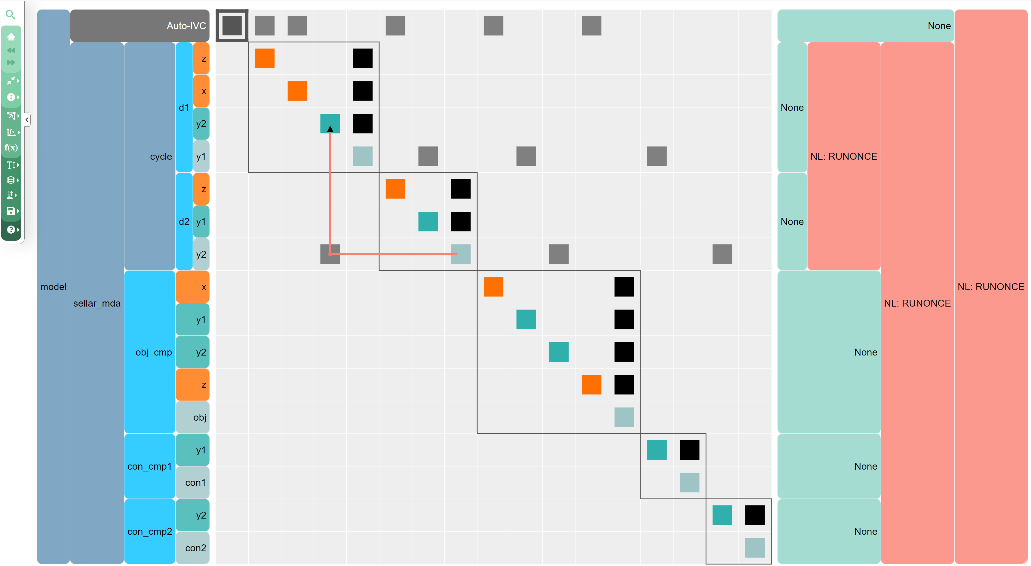
2. Check your data connections within your model. Using solver debug printing might reveal some values are not what you expect. This might be because those variables are not hooked up in your model correctly. You can using the N2 diagram (openmdao n2 model.py, example shown below) to visualize your connections or the openmdao view_connections model.py command-line option to see a text output of your connections. Verify that all of the variables are connected as you expect.
3. Try improving your initial guess for the state values. This is helpful for all solver types, but especially Newton-based methods. You can see if your guess is better or worse by examining the 0th iteration residual when your solve starts. If your initial residual is huge compared to the tolerance you’re asking for and the solver cannot converge the system that far, try to intuitively set up a better initial states vector using your understanding of the physical system you’re modeling. For example, in the case of engine modeling, this means having a reasonable guess for the air mass flow rate through the engine based on the flight condition you’re evaluating.
Sometimes systems have multiple solutions. A simple example to visualize would be a parabola that intersects the x-axis in two places. In the general sense, which solution you should accept is dependent on your model and problem. Maybe anything that satisfies the system of equations is valid, but in most cases there is a more valid solution. An example would be solving for the mass of a component on an aircraft. There might be a valid summation of component masses but one of the components has a negative mass value. That doesn’t make any sense! So using initial guesses close to a physical solution is a great idea to help solver convergence.
from openmdao.test_suite.scripts.circuit_analysis import Circuit

# In this first case, we won't set any guesses for the state values.
# The solver cannot converge the system with the default settings and values.
p = om.Problem()
model = p.model
model.add_subsystem('circuit', Circuit())
p.setup()

nl = model.circuit.nonlinear_solver = om.NewtonSolver(solve_subsystems=False)
nl.options['iprint'] = 2
p.run_model()


# Now, we try again and give better initial guesses.
p = om.Problem()
model = p.model

model.add_subsystem('circuit', Circuit())

p.setup()

nl = model.circuit.nonlinear_solver = om.NewtonSolver(solve_subsystems=False)
nl.options['iprint'] = 2
nl.options['maxiter'] = 25

# set some good initial guesses
p.set_val('circuit.I_in', 0.01, units='A')
p.set_val('circuit.Vg', 0.0, units='V')
p.set_val('circuit.n1.V', 1.)
p.set_val('circuit.n2.V', 0.5)

p.run_model()
=======
circuit
=======
NL: Newton 0 ; 1.37186448e+52 1
NL: Newton 1 ; 5.04690491e+51 0.36788655
NL: Newton 2 ; 1.85668844e+51 0.135340514
NL: Newton 3 ; 6.83050703e+50 0.0497899547
NL: Newton 4 ; 2.51285167e+50 0.0183170546
NL: Newton 5 ; 9.2444433e+49 0.00673859804
NL: Newton 6 ; 3.40090635e+49 0.00247903958
NL: Newton 7 ; 1.25114771e+49 0.00091200532
NL: Newton 8 ; 4.60280413e+48 0.000335514491
NL: Newton 9 ; 1.69330973e+48 0.000123431269
NL: Newton 10 ; 6.22945876e+47 4.54087036e-05
NL: NewtonSolver 'NL: Newton' on system 'circuit' failed to converge in 10 iterations.
=======
circuit
=======
NL: Newton 0 ; 2.63440686 1
NL: Newton 1 ; 10.2098095 3.8755629
NL: Newton 2 ; 3.75604877 1.42576639
NL: Newton 3 ; 1.38179632 0.524518949
NL: Newton 4 ; 0.508340098 0.192961879
NL: Newton 5 ; 0.187006627 0.0709862358
NL: Newton 6 ; 0.0687916876 0.0261127803
NL: Newton 7 ; 0.0253013258 0.00960418306
NL: Newton 8 ; 0.00930113345 0.00353063666
NL: Newton 9 ; 0.00341421321 0.00129600832
NL: Newton 10 ; 0.00124785642 0.000473676423
NL: Newton 11 ; 0.000450327474 0.000170940746
NL: Newton 12 ; 0.000156619343 5.94514635e-05
NL: Newton 13 ; 4.89476723e-05 1.85801491e-05
NL: Newton 14 ; 1.12684364e-05 4.27740931e-06
NL: Newton 15 ; 1.12181954e-06 4.2583382e-07
NL: Newton 16 ; 1.45058216e-08 5.50629509e-09
NL: Newton 17 ; 2.7662285e-12 1.05003845e-12
NL: Newton Converged
4. Try checking the bounds on the state values in your model, if you have any. As mentioned in the immediately previous section, sometimes the solver might try to converge to a non-physical solution. If so, you can change your bounds on your state values to remove this point from the solution space. Or, you might be bounding your problem in a way that there are no valid solutions and you should rethink your bound values.
Additionally, sometimes your solver might “plateau out” or reach a point where the solution cannot be improved further. This looks like the residuals not changing iteration to iteration. This is usually caused by the states hitting a bound. The solver really wants to move past the bound, hence the non-zero residuals, but a bound on a state is preventing it from doing so. If you encounter this, you can change your bounds if it doesn’t negatively impact your problem formulation. You usually need some sort of physical understanding of your model to intelligently change your bounds to reasonable values.
5. This is only for fixed-point iteration methods, like nonlinear block Gauss-Seidel. If your solver is not converging, try adding Aitken relaxation by setting the use_aitken solver option to True. You should turn on Aitken relaxation and see if it helps your model – it does in most cases. This is especially helpful for tightly coupled models.
from openmdao.test_suite.components.sellar_feature import SellarMDA

prob = om.Problem()
model = prob.model

model.add_subsystem('sellar_mda', SellarMDA())
prob.setup()
nlbgs = model.sellar_mda.cycle.nonlinear_solver = om.NonlinearRunOnce()
nlbgs = model.sellar_mda.nonlinear_solver = om.NonlinearBlockGS()
nlbgs.options["iprint"] = 2  # change the print to show the residuals
nlbgs.options["use_aitken"] = True  # Aitken relaxation improves convergence in some cases

prob.run_model()
==========
sellar_mda
==========
NL: NLBGS 1 ; 50.5247285 1
NL: NLBGS 2 ; 3.91711889 0.0775287471
NL: NLBGS 3 ; 0.0744313595 0.00147316694
NL: NLBGS 4 ; 2.9722743e-05 5.88281104e-07
NL: NLBGS 5 ; 1.16801147e-08 2.31176199e-10
NL: NLBGS 6 ; 2.21703753e-10 4.38802462e-12
NL: NLBGS Converged
6. This is only for Newton methods; consult this fantastic doc page which has more detail and more steps for your Newton solver debugging. I don’t have any code snippets to add for this one since the doc page is so fantastic. Definitely check it out!
First check your linear solver to make sure it is converging the derivative values correctly. Because Newton methods depend on the derivative values, if your linear system provides incorrect gradient information it can cause your nonlinear solver to fail.
If your Newton method isn’t converging, try adding a linesearch, such as an ArmijoGoldstein linesearch.
Another consideration is the usage of solve_subsystems, which if True, essentially runs a nonlinear block Gauss-Seidel iteration before starting the Newton solver. This might help put your states in a good spot before attempting the Newton solve.
7. This might take more time to implement, but try reorganizing your model to minimize the amount of subsystems contained within the solver (if you haven’t already). By having only the absolutely necessary subsystems within a solver loop you can drastically reduce computational cost compared to having solvers that iterate across groups unnecessarily. Anecdotally, we once improved speed of a code about 25x by changing where the solver was located within the model hierarchy, which allowed us to use more iterations and then reach convergence. This doesn’t necessarily help convergence but instead allows you to iterate through debugging methods much more quickly.
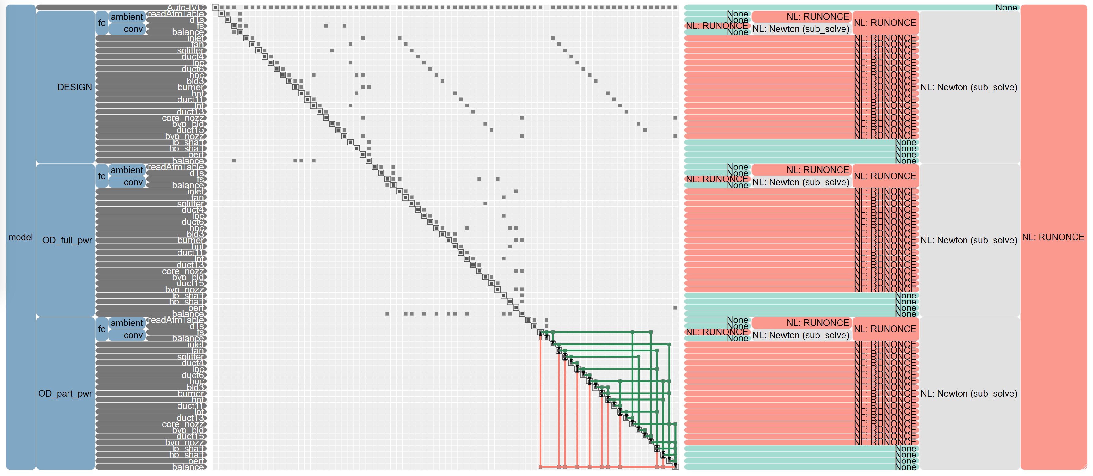
This would be a challenging concept to represent using some sample code, so I will instead show an N2 diagram from a complicated pyCycle engine model. There’s a lot going on in this diagram, but I want to highlight specifically where the solvers are set in this model.
There are three main groups within this model, DESIGN, OD_full_pwr, and OD_part_pwr. In the screenshot I have highlighted the coupling within the OD_part_pwr group in the bottom center of the image. There are many coupled components or groups that feed back within this group, but there is no feedback to the DESIGN or OD_full_pwr groups. Because of this, there are individual Newton solvers on each of those top-level groups instead of a single top-level Newton solver. This allows each of the groups to be converged individually which results in lower computational cost and potentially more robust convergence.
8. This also might take a bit of time to implement, but try using a nested solver hierarchy. If you’re having issues converging a complicated system, solving smaller subsystems and passing those solved systems up into the larger system might fix your problem. Unfortunately, this might introduce increased computational cost, but it should hopefully increase the robustness of your analysis. [[Nested nonlinear solvers]] goes into much more detail about this.
Again, this is a challenging concept to show with a code snippet. The pyCycle N2 model above is also a good example of nested solvers. On the right hand side of the image you can see the solver setup and within each one of the top-level groups there are instances of nested Newton solvers. These lower level solvers help converge the flow properties before handing off the converged results to the rest of the system and the higher level solvers.
This consideration is really only relevant for pretty complicated models where multiple solvers are needed. In the case of a single set of state values or a limited amount of coupling or implicity between systems, using a nested solver hierarchy would not majorly impact the convergence of the system.
This is a detailed sub-point, but if you have a nested hierarchy, try only using the err_on_non_converge solver option at the top level, not at the sub-levels. This will allow the sub-levels to fail to converge without throwing an error and then your top level solver can try to converge the states. Sometimes your model might be erroring out unnecessarily if you have err_on_non_converge on at sub-levels within your model.
9. Try removing some states from the solver loop. This might seem counterintuitive but I suggest “freezing” some of the states so that they do not change in the solver loop. This will allow you to determine if there is a specific subset of states that is causing the solver to fail.
A physical example would be in the case of floating offshore wind turbine design. Consider the multibody dynamics solver – the thing that resolves how the wind and waves moves the turbine blades, affecting the generator, tower, and floating platform. If you “turn off” the waves (treat the wind turbine as land-based) so that they have no effect on the system, you effectively remove the states associated with that motion. Maybe then your system will converge and you know that you need to focus on the effects introduced by the waves.
Another example is in the case of aerostructural wing design. If your aerostructural solver is not converging, a simple thing to try is to set the moduli of the structures to be much larger (1e9 times bigger) than realistic values, essentially making the structure extremely stiff. This should cause the structural displacements to be 0 given any reasonable force on the wing. Obviously this doesn’t help you converge your system in a realistic case, but if your solver still fails with that setup, then you know something more nefarious is going on.
It greatly helps if you build your problem up piece-by-piece, solving each subpiece as you go along, so you can better understand if any additional physical considerations are causing convergence issues.