Outputted files and how to read them

Note

Please also see this doc page for more info about the Aviary dashboard and the information is contains. We usually expect that users access these reports through the dashboard, though you can also access the html files directly.

Each standard Aviary run generates several output files. Which output files are generated depend on the run options. In this section, we assume that we’ve set max_iter = 50 to ensure convergence. The following screenshots used in this article are all from a run using aircraft_for_bench_GwGm.csv.

First, there is always a sub-folder reports/case_name where case_name is the csv file name. In our case, it is reports/aircraft_for_bench_GwGm. It contains a few HTML files:

• driver_scaling_report.html

• inputs.html

• n2.html

• opt_report.html

• total_coloring.html

• traj_linkage_report.html

• traj_results_report.html

File driver_scaling_report.html

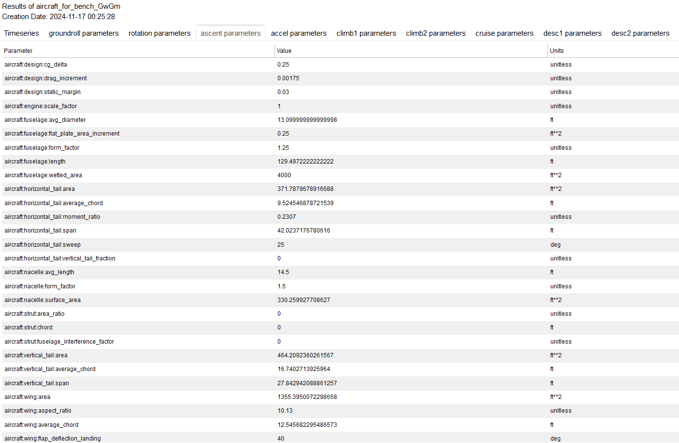
This file is a summary of driver scaling information. After all design variables, objectives, and constraints are declared and the problem has been set up, this report presents all the design variables and constraints in all phases as well as the objectives. The file is divided to three blocks: Design Variables, Constraints, and Objectives. It contains the following columns: name, size, indices, driver value and units, model value and units, ref, ref0, scaler, adder, etc. It also shows Jacobian Info - responses with respect to design variables (DV). A screen shot of design variables is shown here:

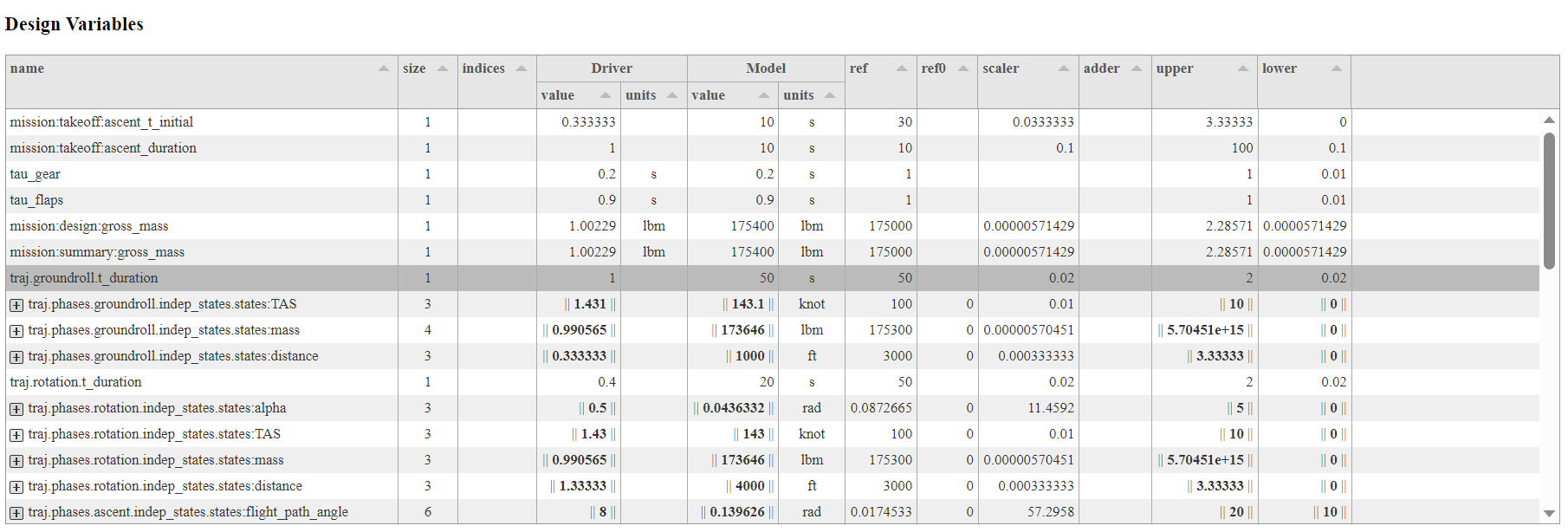
This file is needed when you are debugging. New users can skip it.

File inputs.html

File inputs.html is a sortable and filterable input report of input variables in different phases. It contains all the input variables (with possibly duplicate names for different phases) but only shows those in Source is IVC (abbreviation for IndepVarComp) on opening up. Users can choose to show other inputs by selecting and deselecting this checkbox. Users can filter their inputs by input name, source name, units, shape, tags, values (Val), or design variables (Source is DV). Here is a screen shot (top part) when it is opened:

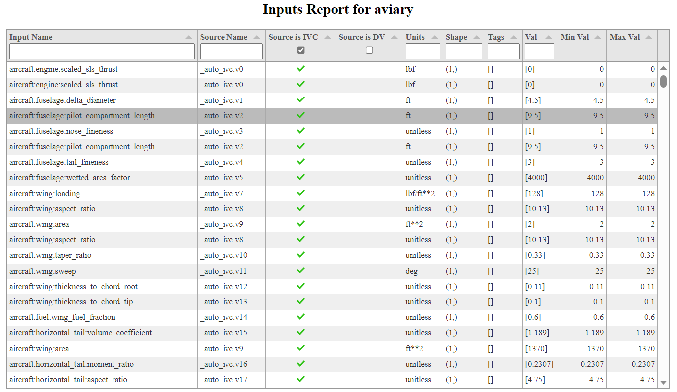
New users can choose to use input_list.txt instead (see below) if settings:verbosity is set to 2 or higher. Note that this file lives in the current folder.

File n2.html

N2, sometimes referred to as an eXtended Design Structure Matrix (XDSM), is a powerful tool for understanding your model in OpenMDAO. It is an N-squared diagram in the shape of a matrix representing functional or physical interfaces between system elements. It can be used to systematically identify, define, tabulate, design, and analyze functional and physical interfaces.

Note

We strongly recommend that you understand N2 diagrams well, especially if you are debugging a model or adding external subsystems. Here is a doc page featuring an informative video on how to use N2 diagrams effectively. MDO lab has another resource for learning about N2 and XDSM.

Here is a screenshot of an N2 diagram after we run aviary run_mission models/aircraft/test_aircraft/aircraft_for_bench_GwGm.csv.

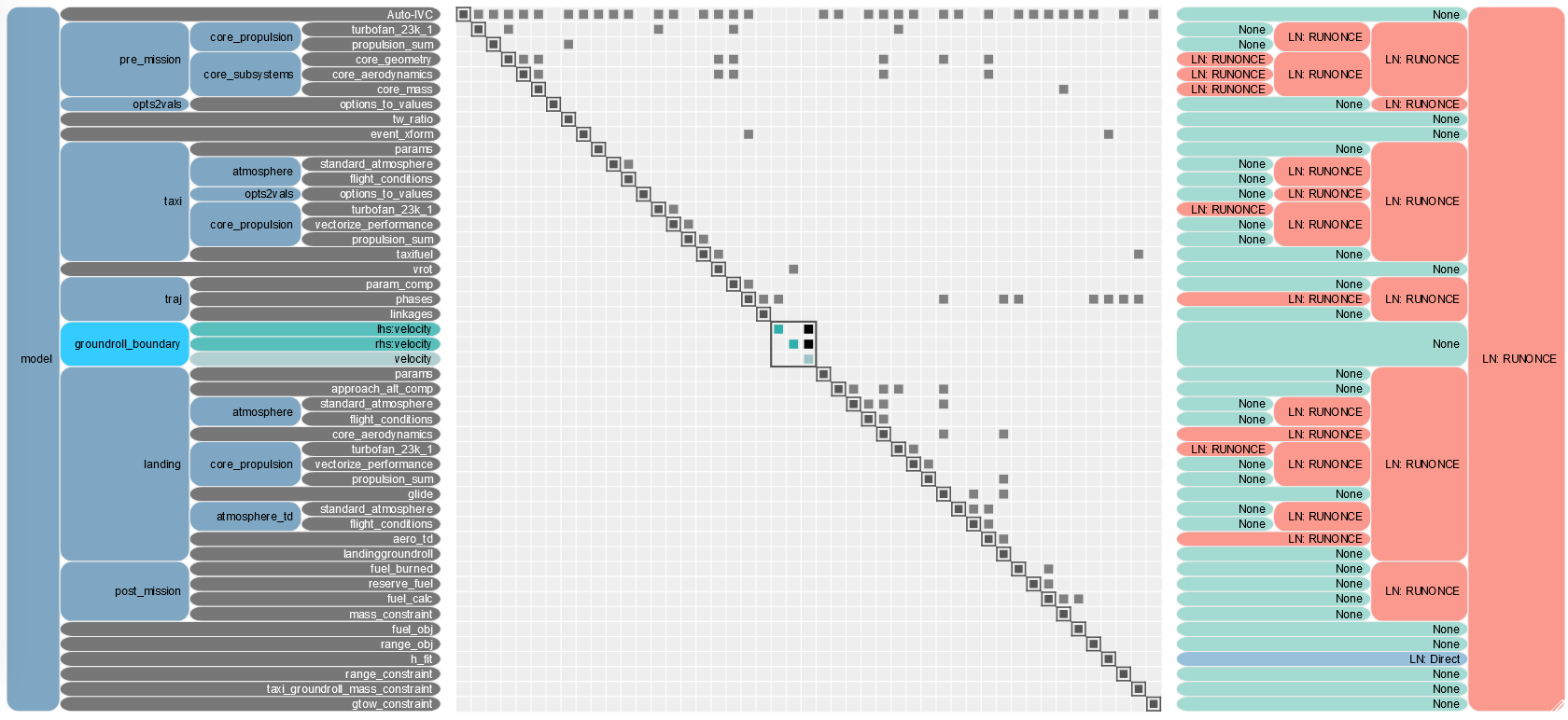
At level 1, we are interested in the phases, so let us Hide solvers. So from model, zoom into traj, then into phases. We see the phases from groundroll to desc2 as expected. To see how those phases are connected, we click on Show all connections in view. Here is what we see:

The solid arrow connections show how outputs of one phase feed as inputs to the next. As you can see, the input of each phase is linked from the previous phase and its output is linked to the next phase. This is pretty much what we expect. The dashed arrows are links to and/or from other places not in the view. If you are curious where those links go, you must zoom out. This can be done by clicking the vertical bar on the left. Let us click it twice. Here is what we get:

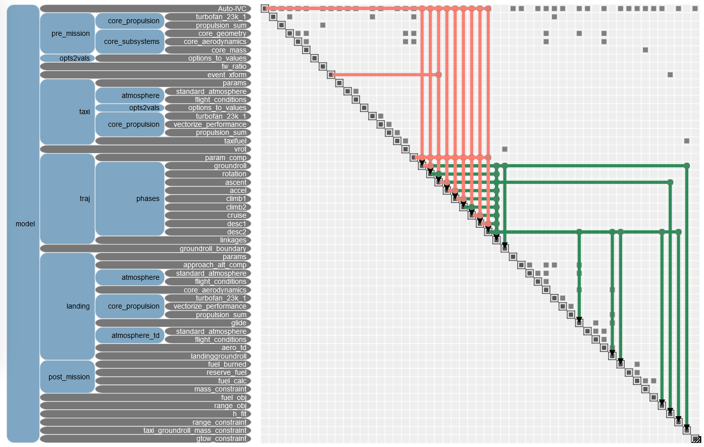
For TWO_DEGREES_OF_FREEDOM missions, there is a takeoff subsystem (including taxi phase) within pre_mission. For ENERGY_STATE missions, there is a takeoff subsystem within pre_mission in which a takeoff phase is added. It is added after static_analysis in add_pre_mission_systems() method.

Similarly, there is a landing phase within post_mission.

File opt_report.html

This file is OpenMDAO Optimization Report. All values are in unscaled, physical units. On the top is a summary of the optimization, followed by the objective, design variables, constraints, and optimizer settings. Here is a screenshot:

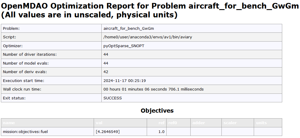
This file is important when dissecting optimal results produced by Aviary.

Coloring files

There is a sub-folder coloring_files. Those are used internally by OpenMDAO for derivative computation. Users should generally skip those files.

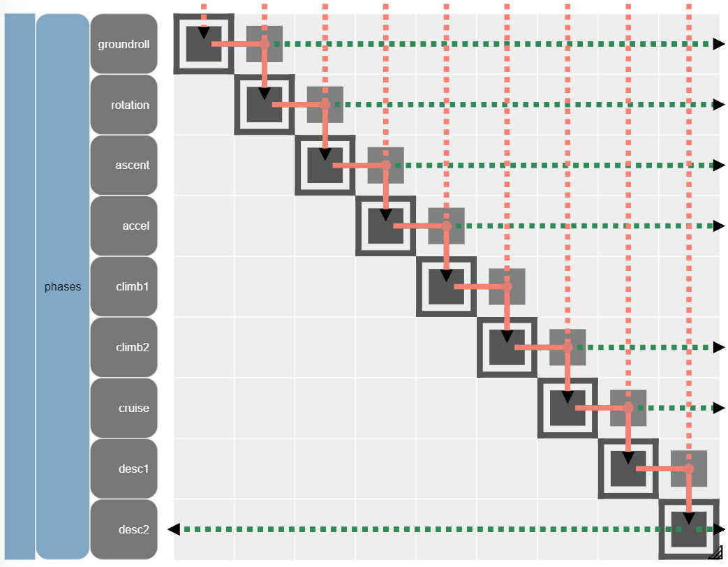
File traj_linkage_report.html

This is a dymos linkage report in a customized N2 diagram. It provides a report detailing how phases are linked together via constraint or connection. It can be used to identify errant linkages between fixed quantities.

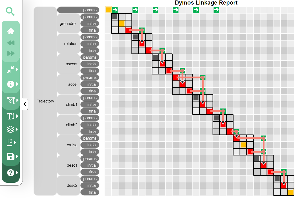
We clearly see how those mission phases are linked.

File traj_results_report.html

Note

This is one of the most important files produced by Aviary. It will help you visualize and understand the optimal trajectory produced by Aviary.

This file contains timeseries and phase parameters in different tabs. For our aircraft_for_bench_GwGm run, they are: groundroll, rotation, ascent, accel, climb1, climb2, cruise, desc1, and desc2 parameters. On the timeseries tab, users can select which phases to view. The following are the top of timeseries tab and ascent parameters tab:

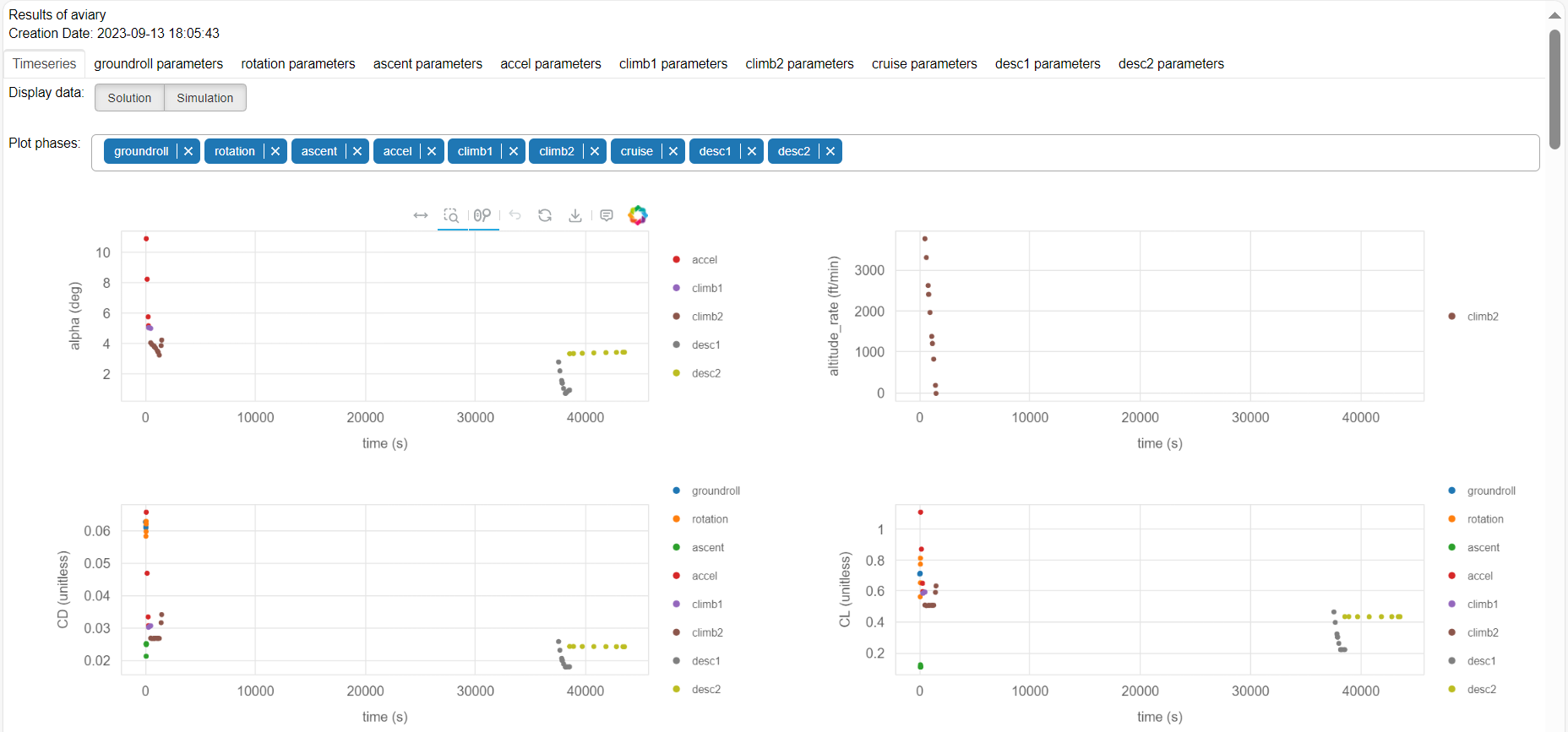
Let’s find the altitude chart. Move the cursor to the top of climb2. We see that the aircraft climbs to 37500 feet at 1200 second. Then it enters to cruise phase. At 28090 second, it starts descent from 40000 feet.

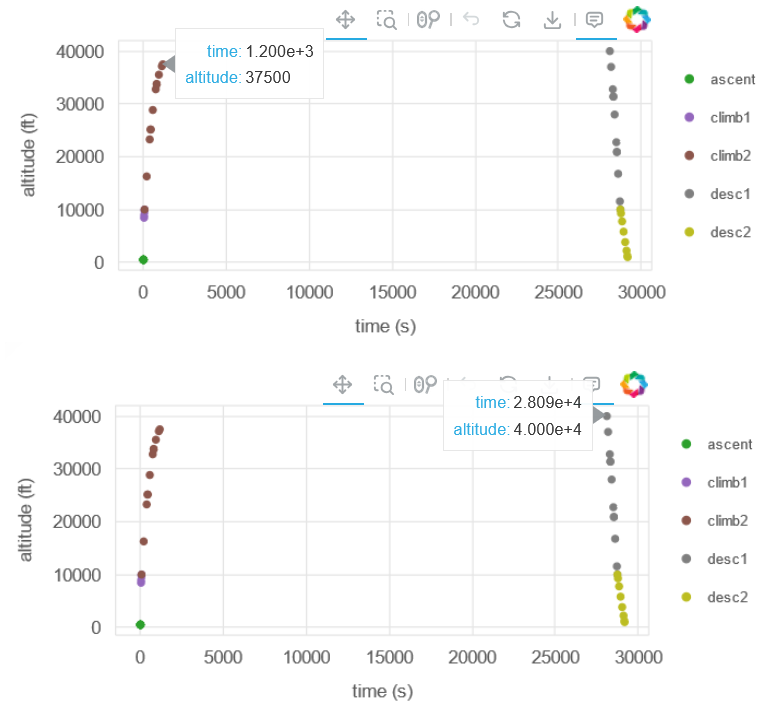
Let’s switch to ascent tab. We see the following:

This file is quite important. Users should play with it and try to grasp all possible features. For example, you can hover the mouse over the solution points to see solution value; you can save the interesting images; you can zoom into a particular region for details, etc.

Optimizer output

If IPOPT is the optimizer, IPOPT.out is generated. If SLSQP is the optimizer and pyOptSparseDriver is the driver, SLSQP.out is generated. Generally speaking, IPOPT and SNOPT converge Aviary optimization problems better than SLSQP, but SLSQP is bundled with Scipy by default, making it more widely available.

SQLite database file

There is a .db file created after run called {glue:md}’problem_history.db’ in the report directory. This is an SQLite database file. Our run is recorded into this file. You generally shouldn’t need to parse through this file on your own, but it is available if you’re seeking additional problem information.

Plain text inputs and outputs

If VERBOSITY is set to 2 (VERBOSE) or higher, input_list.txt and output_list.txt are generated. We recommend this parameter be set to 1 (BRIEF) for beginners. See Coding Standards for more details.

Let us look at input_list.txt:

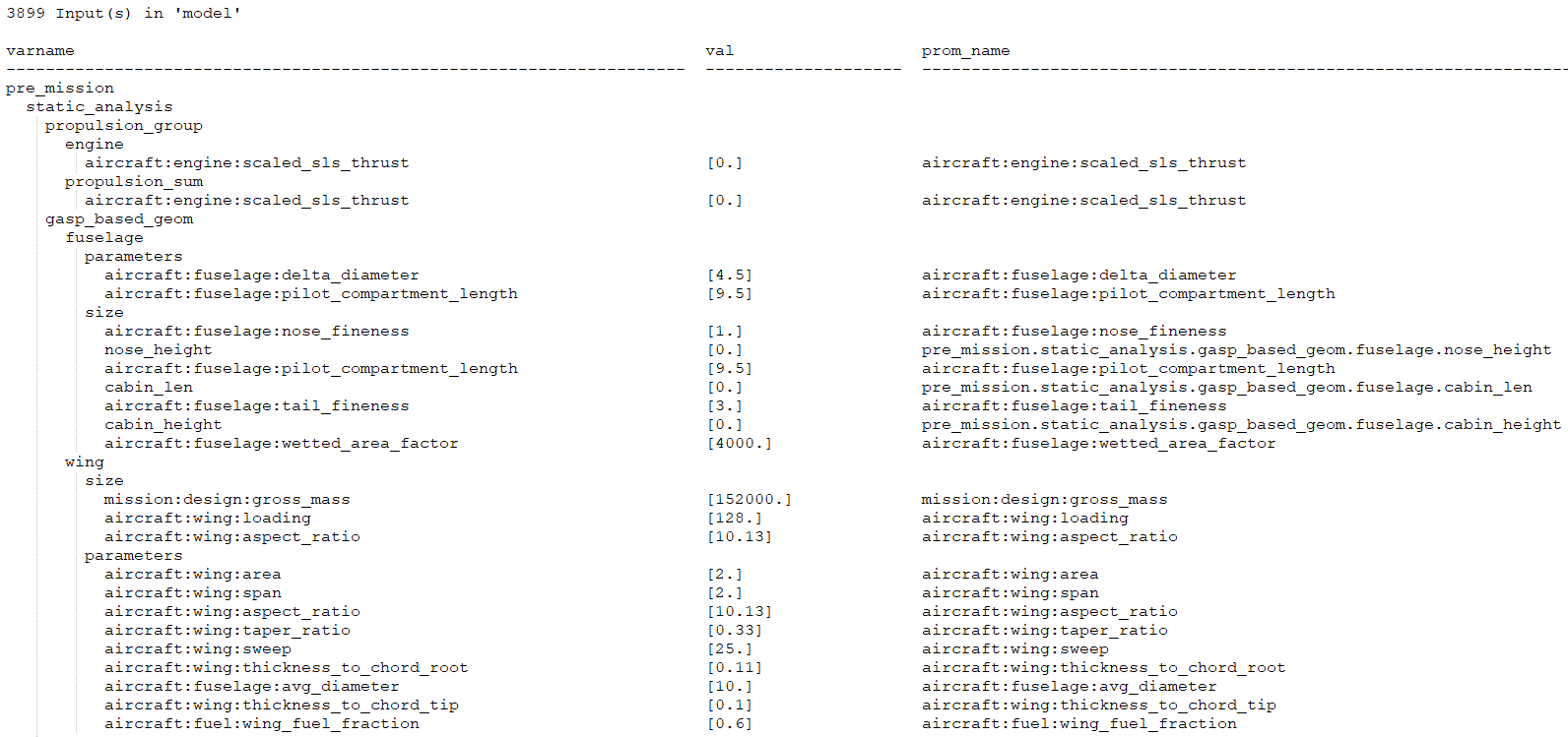
In this screenshot, we see a tree structure. There are three columns. The left column is a list of variable names. The middle column is the value and the right column is the promoted variable name. pre_mission is a phase, static_analysis is a subgroup which contains other subcomponents (e.g. propulsion_group). engine is a component under which is a list of input variables (e.g. aircraft:engine:scaled_sls_thrust).

An input variable can appear under different phases and within different components. Note that its values can be different because its value has been updated during the computation. On the top-left corner is the total number of inputs. That number counts the duplicates because one variable can appear in different phases. Aviary variable structure are discussed in Understanding the Variable Hierarchy and Understanding the Variable Metadata.

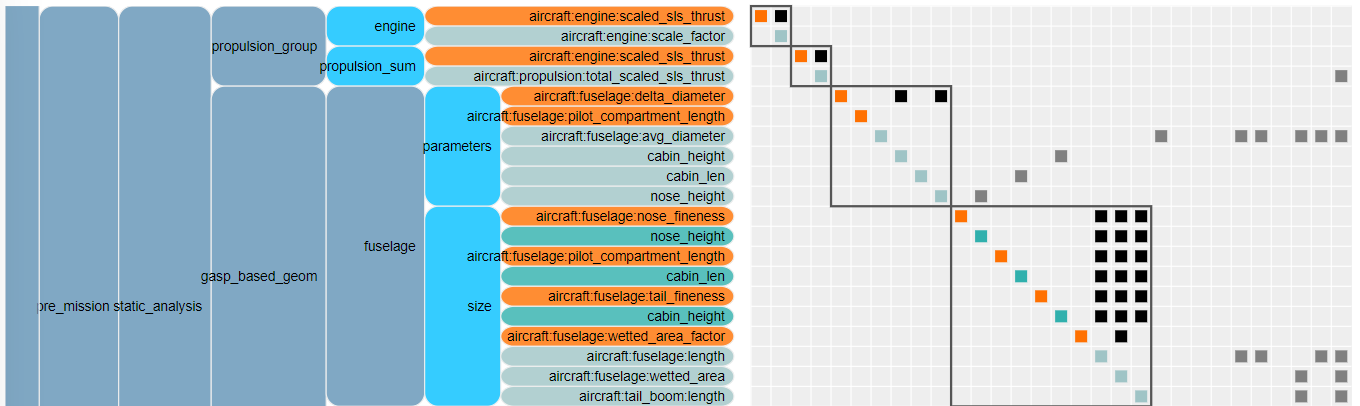
If you zoom the N2 diagram into propulsion_group and gasp_based_geom, you see the exact same tree structure:

File output_list.txt follows the same pattern. But there is another tree for implicit outputs. That helps when debugging is needed.

Additional messages

When Aviary is run, some messages are printed on the command line and they are important. For example, the following constraint report tells us whether our desired constraints are met:

--- Constraint Report [traj] ---
    --- groundroll ---
        None
    --- rotation ---
        [final]   0.0000e+00 == normal_force [lbf]
    --- ascent ---
        [final]   5.0000e+02 == altitude [ft]
        [path]    0.0000e+00 <= load_factor <= 1.1000e+00  [unitless]
        [path]    0.0000e+00 <= fuselage_pitch <= 1.5000e+01  [deg]
    --- accel ---
        [final]   2.5000e+02 == EAS [kn]
    --- climb1 ---
        [final]   1.0000e+04 == altitude [ft]
    --- climb2 ---
        [final]   3.7500e+04 == altitude [ft]
        [final]   1.0000e-01 <= altitude_rate  [ft/min]
        [final]   8.0000e-01 == mach [unitless]
    --- cruise ---
        None
    --- desc1 ---
        [final]   1.0000e+04 == altitude [ft]
    --- desc2 ---
        [final]   1.0000e+03 == altitude [ft]