Mission Analysis#
This page will detail all of the mission implementation and theory details for different ODEs, including EnergyState and 2DOF.
What is a mission in Aviary?#
In the simplest terms, the mission in Aviary is the trajectory that the aircraft flies. Usually this is from takeoff to landing and includes everything in between, depending on the aircraft you’re modeling. For a commercial airliner the mission profile is generally straightforward, featuring climb, cruise, and descent phases. For military craft or non-conventional flight profiles, these missions might also include acceleration, dash, hover, or other phases. A “mission” can also mean a subpart of a more complete mission if you’re studying a portion of the complete flight profile, e.g. focusing on the design of the climb portion of a full mission.
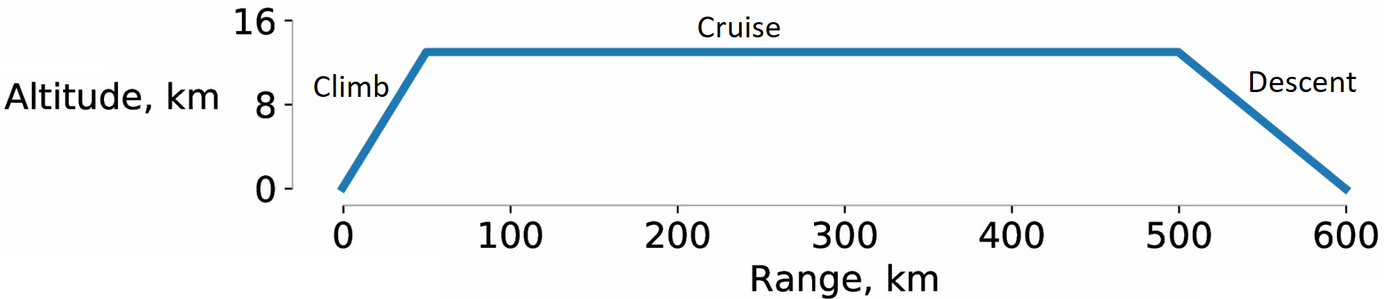
Within Aviary, missions are made up of “phases”. These phases help separate different subparts of the mission into meaningful sections. For example, you might have a climb phase, a cruise phase, and a descent phase. If you wanted to climb first at a specific rate-of-climb, then after that climb to a specific altitude at some fixed Mach number, those would be two separate phases within the mission. An extremely simple mission, showing its climb, cruise, and descent phases, is shown below.
Breaking the mission down into phases allows us to have more control over the control schemes, constraints, and modeling options for each of the flight phases. For example, the climb portion of the flight might feature a nonlinear optimal flight path, whereas the cruise phase is simpler because you might be flying at a constant altitude. By having separate phases for these mission subparts, we can dedicate more care and computational resources to the more “interesting” portions of the flight.
Types of mission models#
There are a few different types of mission modeling methods available in Aviary. At the heart of each mission is the “ODE” (ordinary differential equations) which include the “EOM” (equations of motion). These EOMs describe how the aircraft moves through the air based on the forces the aircraft is experiencing.
Here, I want to be very careful about terminology. I’ll discuss different EOMs and what they mean for the aircraft modeling assumptions. You can use any type of EOM to model any arbitrary mission; the mission profile does not have to follow a certain shape or path. When we discuss “mission modeling,” we are more talking about the assumptions that go into how forces on the aircraft are balanced.
In this section I’ll discuss states, controls, and a few other specialized terms from trajectory modeling and optimization.
There are many resources where these definitions are discussed, but I suggest looking at the Dymos docs which has some very clear explanations for these terms.
Having a basic understanding of some control theory lingo will be helpful for understanding Aviary’s mission formulations.
Energy-state approximation#
The energy-state approximation is a method of describing an aircraft’s energy-state based on its combined kinetic and potential energy. This is a relatively simple EOM model for an aircraft because it does not consider the aircraft’s flight path angle (using small-angle approximations), and treats the aircraft as a point mass without rotational degrees of freedom. Instead, we only care about the aircraft’s current speed and current altitude, as that is all we need to calculate its combined energy. The aircraft is then modeled in such a way that this energy can be instantaneously transferred between the kinetic and potential realms. This is, of course, not exactly physically accurate, but allows us to model the aircraft’s mission in a less computationally expensive manner.
Here is the equation relating altitude \(h\) to energy \(E\) and velocity \(V\), along with the gravitational constant \(g\):
Through this approximation, the only state variable is the energy \(E\) and \(V\) can be considered a control variable.
An excellent introduction to this type of aircraft modeling is Rutowski’s 1953 “Energy Approach to the General Aircraft Performance Problem”.
Two-degrees-of-freedom#
The 2DOF EOM is a bit more detailed than the energy-state approximation as it considers the x-y movement of the aircraft. This means that we need some notion of the aircraft’s flight path heading and speed to obtain its change in the x- and y-directions. The 2DOF model is easily visualized as a force balance on the aircraft, where the acceleration in any direction is calculated by the forces acting on the aircraft and its current mass. This allows us to find the acceleration (change in velocities) in both the x- and y-directions, which we then integrate through the mission to obtain the x-y flight profile.
The unsteady aircraft equations of motion for 2D planar flight are:
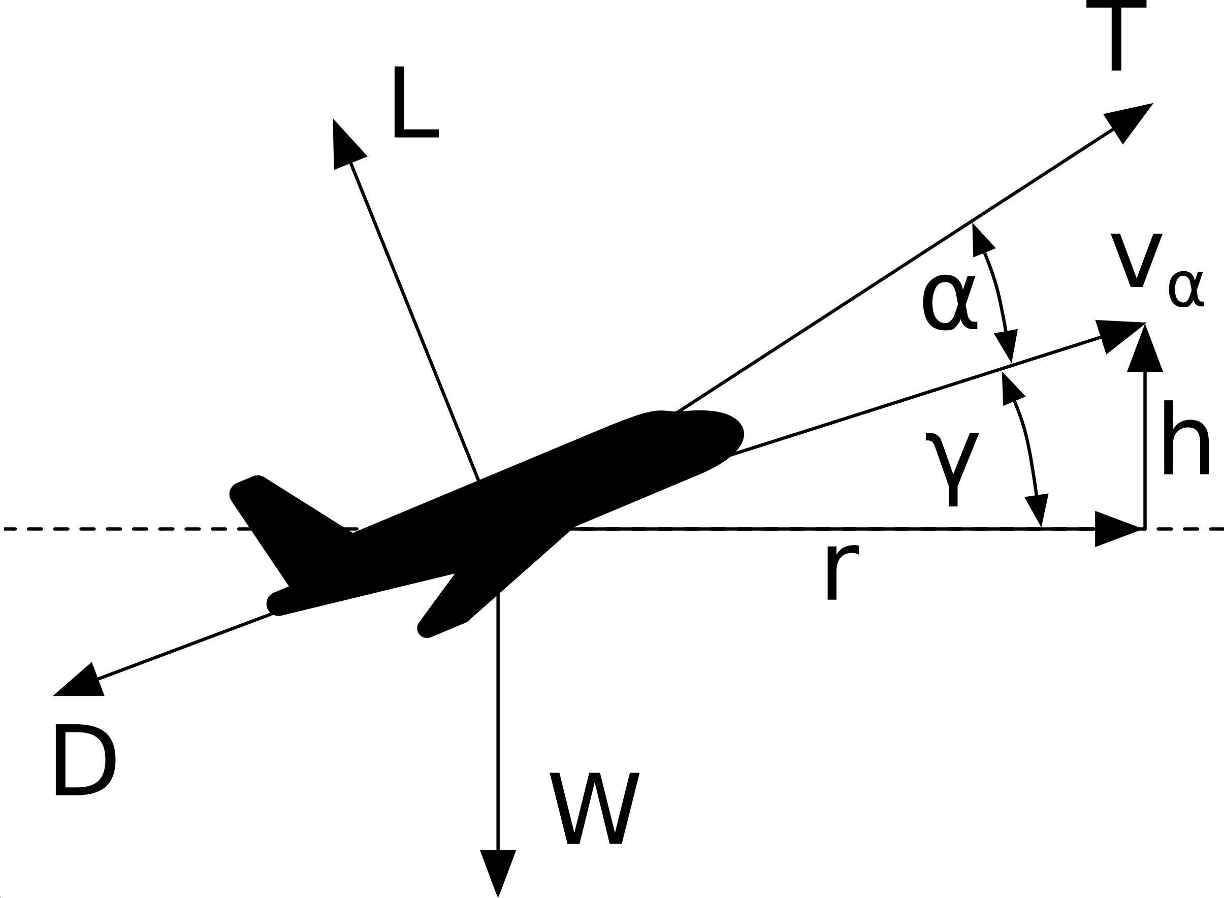
where \(L\), \(D\), \(T\), and \(W\) are the forces of lift, drag, thrust, and weight respectively, \(m\) is the mass of the aircraft, \(V\) is the aircraft velocity, \(\gamma\) is the flight-path angle, \(h\) is the altitude, \(x\) is the horizontal distance, and \(\alpha\) is the angle of attack.
The following figure shows how these forces are oriented relative to an aircraft in flight.