The Length-Constrained Brachistochrone#
Things you’ll learn through this example
How to connect the outputs from a trajectory to a downstream system.
This is a modified take on the brachistochrone problem. In this instance, we assume that the quantity of wire available is limited. Now, we seek to find the minimum time brachistochrone trajectory subject to a upper-limit on the arclength of the wire.
The most efficient way to approach this problem would be to treat the arc-length \(S\) as an integrated state variable. In this case, as is often the case in real-world MDO analyses, the implementation of our arc-length function is not integrated into our pseudospectral approach. Rather than rewrite an analysis tool to accommodate the pseudospectral approach, the arc-length analysis simply takes the result of the trajectory in its entirety and computes the arc-length constraint via the trapezoidal rule:\
The OpenMDAO component used to compute the arclength is defined as follows:
import numpy as np

from openmdao.api import ExplicitComponent


class ArcLengthComp(ExplicitComponent):

    def initialize(self):

        self.options.declare('num_nodes', types=(int,))

    def setup(self):
        nn = self.options['num_nodes']

        self.add_input('x', val=np.ones(nn), units='m', desc='x at points along the trajectory')
        self.add_input('theta', val=np.ones(nn), units='rad',
                       desc='wire angle with vertical along the trajectory')

        self.add_output('S', val=1.0, units='m', desc='arclength of wire')

        self.declare_partials(of='S', wrt='*', method='cs')

    def compute(self, inputs, outputs, discrete_inputs=None, discrete_outputs=None):

        x = inputs['x']
        theta = inputs['theta']

        dy_dx = -1.0 / np.tan(theta)
        dx = np.diff(x)
        f = np.sqrt(1 + dy_dx**2)

        # trapezoidal rule
        fxm1 = f[:-1]
        fx = f[1:]
        outputs['S'] = 0.5 * np.dot(fxm1 + fx, dx)
Note
In this example, the number of nodes used to compute the arclength is needed when building the problem.
The transcription object is initialized and its attribute grid_data.num_nodes is used to provide the number of total nodes (the number of points in the timeseries) to the downstream arc length calculation.
import openmdao.api as om
import dymos as dm
import matplotlib.pyplot as plt
from dymos.examples.brachistochrone.brachistochrone_ode import BrachistochroneODE
MAX_ARCLENGTH = 11.9
OPTIMIZER = 'SLSQP'
p = om.Problem(model=om.Group())
p.add_recorder(om.SqliteRecorder('length_constrained_brach_sol.db'))
if OPTIMIZER == 'SNOPT':
p.driver = om.pyOptSparseDriver()
p.driver.options['optimizer'] = OPTIMIZER
p.driver.opt_settings['Major iterations limit'] = 1000
p.driver.opt_settings['Major feasibility tolerance'] = 1.0E-6
p.driver.opt_settings['Major optimality tolerance'] = 1.0E-5
p.driver.opt_settings['iSumm'] = 6
p.driver.opt_settings['Verify level'] = 3
else:
p.driver = om.ScipyOptimizeDriver()
p.driver.declare_coloring()
# Create the transcription so we can get the number of nodes for the downstream analysis
tx = dm.Radau(num_segments=20, order=3, compressed=False)
traj = dm.Trajectory()
phase = dm.Phase(transcription=tx, ode_class=BrachistochroneODE)
traj.add_phase('phase0', phase)
p.model.add_subsystem('traj', traj)
phase.set_time_options(fix_initial=True, duration_bounds=(.5, 10))
phase.add_state('x', units='m', rate_source='xdot', fix_initial=True, fix_final=True)
phase.add_state('y', units='m', rate_source='ydot', fix_initial=True, fix_final=True)
phase.add_state('v', units='m/s', rate_source='vdot', fix_initial=True, fix_final=False)
phase.add_control('theta', units='deg', lower=0.01, upper=179.9,
continuity=True, rate_continuity=True)
phase.add_parameter('g', units='m/s**2', opt=False, val=9.80665)
# Minimize time at the end of the phase
phase.add_objective('time', loc='final', scaler=1)
# p.model.options['assembled_jac_type'] = top_level_jacobian.lower()
# p.model.linear_solver = DirectSolver(assemble_jac=True)
# Add the arc length component
p.model.add_subsystem('arc_length_comp',
subsys=ArcLengthComp(num_nodes=tx.grid_data.num_nodes))
p.model.connect('traj.phase0.timeseries.theta', 'arc_length_comp.theta')
p.model.connect('traj.phase0.timeseries.x', 'arc_length_comp.x')
p.model.add_constraint('arc_length_comp.S', upper=MAX_ARCLENGTH, ref=1)
p.setup(check=True)
phase.set_time_val(initial=0.0, duration=2.0)
phase.set_state_val('x', [0, 10])
phase.set_state_val('y', [10, 5])
phase.set_state_val('v', [0, 9.9])
phase.set_control_val('theta', [5, 100])
phase.set_parameter_val('g', 9.80665)
p.run_driver()
p.record(case_name='final')
# Generate the explicitly simulated trajectory
exp_out = traj.simulate()
# Extract the timeseries from the implicit solution and the explicit simulation
x = p.get_val('traj.phase0.timeseries.x')
y = p.get_val('traj.phase0.timeseries.y')
t = p.get_val('traj.phase0.timeseries.time')
theta = p.get_val('traj.phase0.timeseries.theta')
x_exp = exp_out.get_val('traj.phase0.timeseries.x')
y_exp = exp_out.get_val('traj.phase0.timeseries.y')
t_exp = exp_out.get_val('traj.phase0.timeseries.time')
theta_exp = exp_out.get_val('traj.phase0.timeseries.theta')
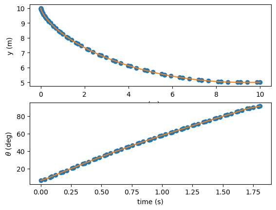
fig, axes = plt.subplots(nrows=2, ncols=1)
axes[0].plot(x, y, 'o')
axes[0].plot(x_exp, y_exp, '-')
axes[0].set_xlabel('x (m)')
axes[0].set_ylabel('y (m)')
axes[1].plot(t, theta, 'o')
axes[1].plot(t_exp, theta_exp, '-')
axes[1].set_xlabel('time (s)')
axes[1].set_ylabel(r'$\theta$ (deg)')
plt.show()
INFO: checking out_of_order...
INFO: out_of_order check complete (0.000264 sec).
INFO: checking system...
INFO: system check complete (0.000018 sec).
INFO: checking solvers...
INFO: solvers check complete (0.000149 sec).
INFO: checking dup_inputs...
INFO: dup_inputs check complete (0.000053 sec).
INFO: checking missing_recorders...
INFO: missing_recorders check complete (0.000003 sec).
INFO: checking unserializable_options...
INFO: unserializable_options check complete (0.001125 sec).
INFO: checking comp_has_no_outputs...
INFO: comp_has_no_outputs check complete (0.000038 sec).
INFO: checking auto_ivc_warnings...
INFO: auto_ivc_warnings check complete (0.000004 sec).
Jacobian shape: (220, 296)  (2.35% nonzero)
FWD solves: 4   REV solves: 17
Total colors vs. total size: 21 vs 220  (90.45% improvement)

Sparsity computed using tolerance: 1e-25.
Dense total jacobian for Problem 'problem' was computed 3 times.
Time to compute sparsity:   0.2873 sec
Time to compute coloring:   0.2463 sec
Memory to compute coloring:   0.7461 MB
Coloring created on: 2026-05-13 14:57:57
Optimization terminated successfully    (Exit mode 0)
            Current function value: 1.808598520786358
            Iterations: 5
            Function evaluations: 5
            Gradient evaluations: 5
Optimization Complete
-----------------------------------
/home/runner/work/dymos/dymos/.openmdao-pixi/.pixi/envs/dev/lib/python3.13/site-packages/openmdao/visualization/opt_report/opt_report.py:611: UserWarning: Attempting to set identical low and high ylims makes transformation singular; automatically expanding.
  ax.set_ylim([ymin_plot, ymax_plot])
Simulating trajectory traj
Done simulating trajectory traj