Cart-Pole Optimal Control

Cart-Pole Optimal Control#

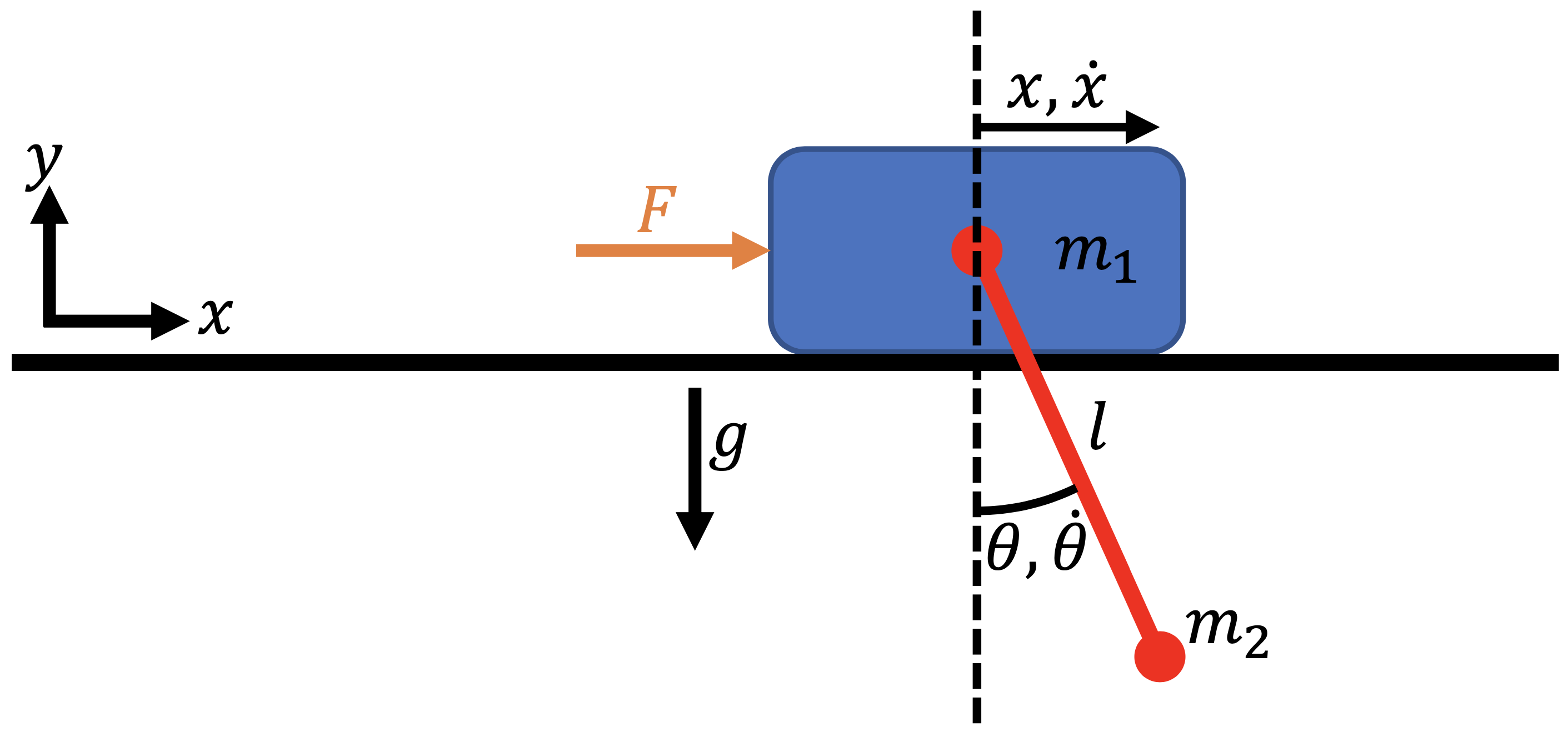
This example is authored by Shugo Kaneko and Bernardo Pacini of the MDO Lab. The cart-pole problem is an instructional case described in An introduction to trajectory optimization: How to do your own direct collocation [Kel17], and is adapted to work within Dymos. We consider a pole that can rotate freely attached to a cart, on which we can exert an external force (control input) in the \(x\)-direction.

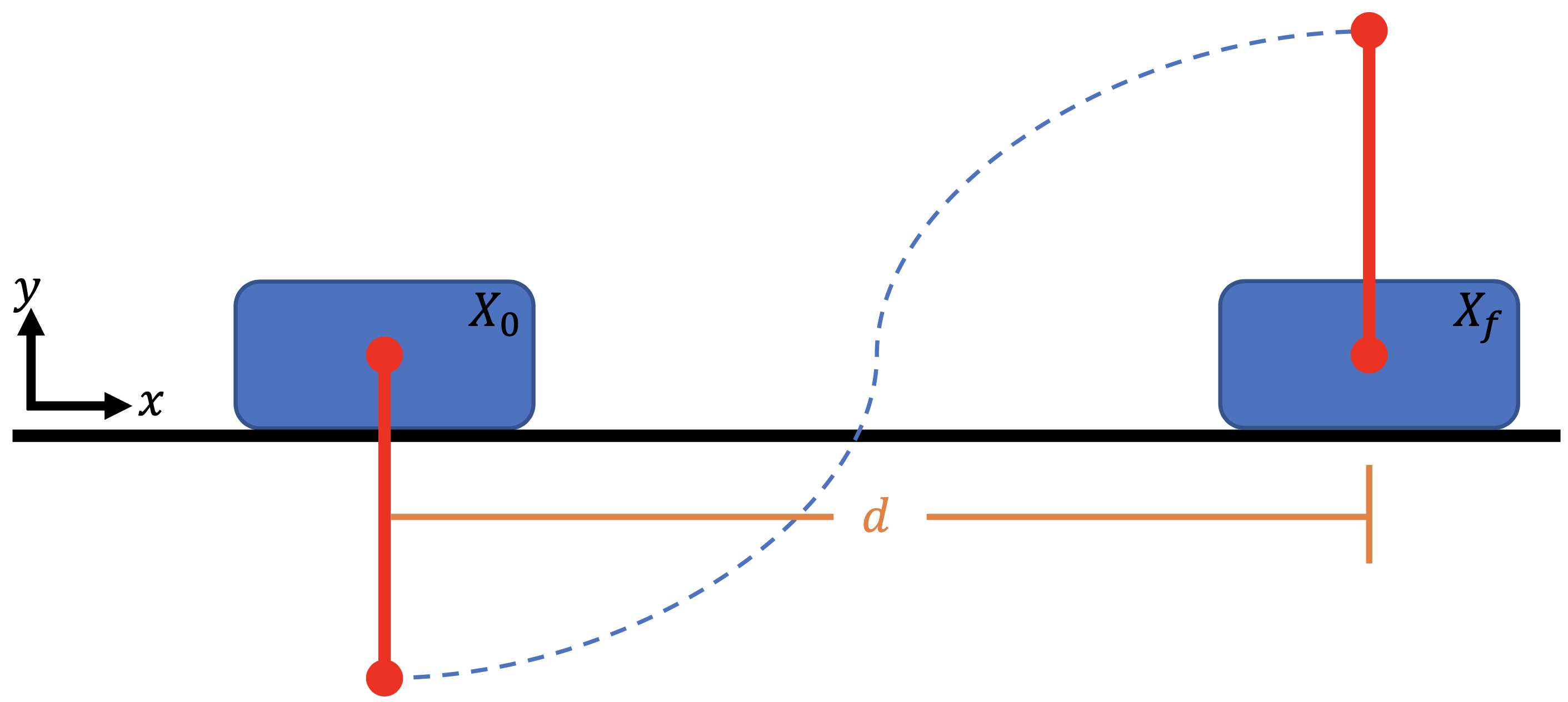
Our goal is to bring the cart-pole system from an initial state to a terminal state with minimum control efforts. The initial state is the stable stationary point (the cart at a stop with the pole vertically down), and the terminal state is the unstable stationary state (the cart at a stop but with the pole vertically up). Friction force is ignored to simplify the problem.

Cart-pole optimal control from the initial state to the terminal state.

Trajectory Optimization Problem#

We use the following quadratic objective function to approximately minimize the total control effort:

(86)#\[\begin{equation} J = \int_{t_0}^{t_f} F(t)^2 dt ~~ \rightarrow ~ \min \end{equation}\]

where \(F(t)\) is the external force, \(t_0\) is the initial time, and \(t_f\) is the final time.

Dynamics#

The equations of motion of the cart-pole system are given by

(87)#\[\begin{equation} \begin{bmatrix} \ddot{x} \\ \ddot{\theta} \end{bmatrix} = \begin{bmatrix} \cos \theta & \ell \\ m_1 + m_2 & m_2 \ell \cos \theta \end{bmatrix}^{-1} \begin{bmatrix} -g \sin \theta \\ F + m_2 \ell \dot{\theta}^2 \sin \theta \end{bmatrix} \end{equation}\]

where \(x\) is the cart location, \(\theta\) is the pole angle, \(m_1\) is the cart mass, \(m_2\) is the pole mass, and \(\ell\) is the pole length.

Schematic of the cart-pole system.

Now, we need to convert the equations of motion, which are a second-order ODE, to a first-order ODE. To do so, we define our state vector to be \(X = [x, \dot{x}, \theta, \dot{\theta}]^T\). We also add an “energy” state \(e\) and set \(\dot{e} = F^2\) to keep track of the accumulated control input. By setting setting \(e_0 = 0\), the objective function is equal to the final value of the state \(e\):

(88)#\[\begin{equation} J = \int_{t_0}^{t_f} \dot{e} ~dt = e_f \end{equation}\]

To summarize, the ODE for the cart-pole system is given by

(89)#\[\begin{equation} \begin{bmatrix} \dot{x} \\ \dot{\theta} \\ \ddot{x} \\ \ddot{\theta} \\ \dot{e} \end{bmatrix} = f \left( \begin{bmatrix} x \\ \theta \\ \dot{x} \\ \dot{\theta} \\ e \end{bmatrix} \right)= \begin{bmatrix} \dot{x} \\ \dot{\theta} \\ \frac{-m_2 g \sin \theta \cos \theta - (F + m_2 \ell \dot{\theta}^2 \sin \theta)}{m_2 \cos^2 \theta - (m_1 + m_2)} \\ \frac{(m_1 + m_2) g \sin \theta + \cos \theta (F + m_1 \ell \dot{\theta}^2 \sin \theta)}{m_2 \ell \cos^2 \theta - (m_1 + m_2) \ell} \\ F^2 \\ \end{bmatrix} \end{equation}\]

Initial and terminal conditions#

The initial state variables are all zero at \(t_0 = 0\), and the final conditions at time \(t_f\) are

(90)#\[\begin{align} x_f &= d \\ \dot{x}_f &= 0 \\ \theta_f &= \pi \\ \dot{\theta_f} &= 0 \end{align}\]

Parameters#

The fixed parameters are summarized as follows.

Parameter	Value	Units	Description
\(m_1\)	1.0	kg	Cart mass
\(m_2\)	0.3	kg	Pole mass
\(\ell\)	0.5	m	Pole length
\(d\)	2	m	Cart target location
\(t_f\)	2	s	Final time

Implementing the ODE#

We first implement the cart-pole ODE as an ExplicitComponent as follows:

import openmdao.api as om
om.display_source("dymos.examples.cart_pole.cartpole_dynamics")

"""
Cart-pole dynamics (ODE)
"""

import numpy as np
import openmdao.api as om


class CartPoleDynamics(om.ExplicitComponent):
    """
    Computes the time derivatives of states given state variables and control inputs.

    Parameters
    ----------
    m_cart : float
        Mass of cart.
    m_pole : float
        Mass of pole.
    l_pole : float
        Length of pole.
    theta : 1d array
        Angle of pole, 0 for vertical downward, positive counter clockwise.
    theta_dot : 1d array
        Angluar velocity of pole.
    f : 1d array
        x-wise force applied to the cart.

    Returns
    -------
    x_dotdot : 1d array
        Acceleration of cart in x direction.
    theta_dotdot : 1d array
        Angular acceleration of pole.
    e_dot : 1d array
        Rate of "energy" state.
    """

    def initialize(self):
        self.options.declare(
            "num_nodes", default=1, desc="number of nodes to be evaluated (i.e., length of vectors x, theta, etc)"
        )
        self.options.declare("g", default=9.81, desc="gravity constant")

    def setup(self):
        nn = self.options["num_nodes"]

        # --- inputs ---
        # cart-pole parameters
        self.add_input("m_cart", shape=(1,), units="kg", desc="cart mass")
        self.add_input("m_pole", shape=(1,), units="kg", desc="pole mass")
        self.add_input("l_pole", shape=(1,), units="m", desc="pole length")
        # state variables. States x, x_dot, energy have no influence on the outputs, so we don't need them as inputs.
        self.add_input("theta", shape=(nn,), units="rad", desc="pole angle")
        self.add_input("theta_dot", shape=(nn,), units="rad/s", desc="pole angle velocity")
        # control input
        self.add_input("f", shape=(nn,), units="N", desc="force applied to cart in x direction")

        # --- outputs ---
        # rate of states (accelerations)
        self.add_output("x_dotdot", shape=(nn,), units="m/s**2", desc="x acceleration of cart")
        self.add_output("theta_dotdot", shape=(nn,), units="rad/s**2", desc="angular acceleration of pole")
        # also computes force**2, which will be integrated to compute the objective
        self.add_output("e_dot", shape=(nn,), units="N**2", desc="square of force to be integrated")

        # ---  partials ---.
        # Jacobian of outputs w.r.t. state/control inputs is diagonal
        # because each node (corresponds to time discretization) is independent
        self.declare_partials(of=["*"], wrt=["theta", "theta_dot", "f"], method="exact", rows=np.arange(nn), cols=np.arange(nn))

        # partials of outputs w.r.t. cart-pole parameters. We will use complex-step, but still declare the sparsity structure.
        # NOTE: since the cart-pole parameters are fixed during optimization, these partials are not necessary to declare.
        self.declare_partials(of=["*"], wrt=["m_cart", "m_pole", "l_pole"], method="cs", rows=np.arange(nn), cols=np.zeros(nn))
        self.set_check_partial_options(wrt=["m_cart", "m_pole", "l_pole"], method="fd", step=1e-7)

    def compute(self, inputs, outputs):
        g = self.options["g"]
        mc = inputs["m_cart"]
        mp = inputs["m_pole"]
        lpole = inputs["l_pole"]
        theta = inputs["theta"]
        omega = inputs["theta_dot"]
        f = inputs["f"]

        sint = np.sin(theta)
        cost = np.cos(theta)
        det = mp * lpole * cost**2 - lpole * (mc + mp)
        outputs["x_dotdot"] = (-mp * lpole * g * sint * cost - lpole * (f + mp * lpole * omega**2 * sint)) / det
        outputs["theta_dotdot"] = ((mc + mp) * g * sint + cost * (f + mp * lpole * omega**2 * sint)) / det
        outputs["e_dot"] = f**2

    def compute_partials(self, inputs, jacobian):
        g = self.options["g"]
        mc = inputs["m_cart"]
        mp = inputs["m_pole"]
        lpole = inputs["l_pole"]
        theta = inputs["theta"]
        theta_dot = inputs["theta_dot"]
        f = inputs["f"]

        # --- derivatives of x_dotdot ---
        # Collecting Theta Derivative
        low = mp * lpole * np.cos(theta) ** 2 - lpole * mc - lpole * mp
        dhigh = (
            mp * g * lpole * np.sin(theta) ** 2 -
            mp * g * lpole * np.cos(theta) ** 2 -
            lpole**2 * mp * theta_dot**2 * np.cos(theta)
        )
        high = -mp * g * lpole * np.cos(theta) * np.sin(theta) - lpole * f - lpole**2 * mp * theta_dot**2 * np.sin(theta)
        dlow = 2.0 * mp * lpole * np.cos(theta) * (-np.sin(theta))

        jacobian["x_dotdot", "theta"] = (low * dhigh - high * dlow) / low**2
        jacobian["x_dotdot", "theta_dot"] = (
            -2.0 * theta_dot * lpole**2 * mp * np.sin(theta) / (mp * lpole * np.cos(theta) ** 2 - lpole * mc - lpole * mp)
        )
        jacobian["x_dotdot", "f"] = -lpole / (mp * lpole * np.cos(theta) ** 2 - lpole * mc - lpole * mp)

        # --- derivatives of theta_dotdot ---
        # Collecting Theta Derivative
        low = mp * lpole * np.cos(theta) ** 2 - lpole * mc - lpole * mp
        dlow = 2.0 * mp * lpole * np.cos(theta) * (-np.sin(theta))
        high = (mc + mp) * g * np.sin(theta) + f * np.cos(theta) + mp * lpole * theta_dot**2 * np.sin(theta) * np.cos(theta)
        dhigh = (
            (mc + mp) * g * np.cos(theta) -
            f * np.sin(theta) +
            mp * lpole * theta_dot**2 * (np.cos(theta) ** 2 - np.sin(theta) ** 2)
        )

        jacobian["theta_dotdot", "theta"] = (low * dhigh - high * dlow) / low**2
        jacobian["theta_dotdot", "theta_dot"] = (
            2.0 *
            theta_dot *
            mp *
            lpole *
            np.sin(theta) *
            np.cos(theta) /
            (mp * lpole * np.cos(theta) ** 2 - lpole * mc - lpole * mp)
        )
        jacobian["theta_dotdot", "f"] = np.cos(theta) / (mp * lpole * np.cos(theta) ** 2 - lpole * mc - lpole * mp)

        # --- derivatives of e_dot ---
        jacobian["e_dot", "theta"] = 0.0
        jacobian["e_dot", "theta_dot"] = 0.0
        jacobian["e_dot", "f"] = 2.0 * f

Building and running the problem#

The following is a runscript of the cart-pole optimal control problem. First, we instantiate the OpenMDAO problem and set up the Dymos trajectory, phase, and transcription.

"""
Cart-pole optimizatio runscript
"""

import numpy as np
import openmdao.api as om
import dymos as dm
from dymos.examples.plotting import plot_results
from dymos.examples.cart_pole.cartpole_dynamics import CartPoleDynamics

p = om.Problem()

# --- instantiate trajectory and phase, setup transcription ---
traj = dm.Trajectory()
p.model.add_subsystem('traj', traj)
phase = dm.Phase(transcription=dm.GaussLobatto(num_segments=40, order=3, compressed=True, solve_segments=False), ode_class=CartPoleDynamics)
# NOTE: set solve_segments=True to do solver-based shooting
traj.add_phase('phase', phase)

<dymos.phase.phase.Phase at 0x7f216f3e1b40>

Next, we add the state variables, controls, and cart-pole parameters.

# --- set state and control variables ---
phase.set_time_options(fix_initial=True, fix_duration=True, duration_val=2., units='s')
# declare state variables. You can also set lower/upper bounds and scalings here.
phase.add_state('x', fix_initial=True, lower=-2, upper=2, rate_source='x_dot', shape=(1,), ref=1, defect_ref=1, units='m')
phase.add_state('x_dot', fix_initial=True, rate_source='x_dotdot', shape=(1,), ref=1, defect_ref=1, units='m/s')
phase.add_state('theta', fix_initial=True, rate_source='theta_dot', shape=(1,), ref=1, defect_ref=1, units='rad')
phase.add_state('theta_dot', fix_initial=True, rate_source='theta_dotdot', shape=(1,), ref=1, defect_ref=1, units='rad/s')
phase.add_state('energy', fix_initial=True, rate_source='e_dot', shape=(1,), ref=1, defect_ref=1, units='N**2*s')  # integration of force**2. This does not have the energy unit, but I call it "energy" anyway.

# declare control inputs
phase.add_control('f', fix_initial=False, rate_continuity=False, lower=-20, upper=20, shape=(1,), ref=0.01, units='N')

# add cart-pole parameters (set static_target=True because these params are not time-depencent)
phase.add_parameter('m_cart', val=1., units='kg', static_target=True)
phase.add_parameter('m_pole', val=0.3, units='kg', static_target=True)
phase.add_parameter('l_pole', val=0.5, units='m', static_target=True)

We set the terminal conditions as boundary constraints and declare the optimization objective.

# --- set terminal constraint ---
# alternatively, you can impose those by setting `fix_final=True` in phase.add_state()
phase.add_boundary_constraint('x', loc='final', equals=1, ref=1., units='m')  # final horizontal displacement
phase.add_boundary_constraint('theta', loc='final', equals=np.pi, ref=1., units='rad')  # final pole angle
phase.add_boundary_constraint('x_dot', loc='final', equals=0, ref=1., units='m/s')  # 0 velocity at the and
phase.add_boundary_constraint('theta_dot', loc='final', equals=0, ref=0.1, units='rad/s')  # 0 angular velocity at the end
phase.add_boundary_constraint('f', loc='final', equals=0, ref=1., units='N')  # 0 force at the end

# --- set objective function ---
# we minimize the integral of force**2.
phase.add_objective('energy', loc='final', ref=100)

Next, we configure the optimizer and declare the total Jacobian coloring to accelerate the derivative computations. We then call the setup method to setup the OpenMDAO problem.

# --- configure optimizer ---
p.driver = om.pyOptSparseDriver()
p.driver.options["optimizer"] = "IPOPT"
# IPOPT options
p.driver.opt_settings['mu_init'] = 1e-1
p.driver.opt_settings['max_iter'] = 600
p.driver.opt_settings['constr_viol_tol'] = 1e-6
p.driver.opt_settings['compl_inf_tol'] = 1e-6
p.driver.opt_settings['tol'] = 1e-5
p.driver.opt_settings['print_level'] = 0
p.driver.opt_settings['nlp_scaling_method'] = 'gradient-based'
p.driver.opt_settings['alpha_for_y'] = 'safer-min-dual-infeas'
p.driver.opt_settings['mu_strategy'] = 'monotone'
p.driver.opt_settings['bound_mult_init_method'] = 'mu-based'
p.driver.options['print_results'] = False

# declare total derivative coloring to accelerate the UDE linear solves
p.driver.declare_coloring()

p.setup(check=False)

--- Constraint Report [traj] ---
    --- phase ---
        [final]   1.0000e+00 == x [m]
        [final]   3.1416e+00 == theta [rad]
        [final]   0.0000e+00 == x_dot [m/s]
        [final]   0.0000e+00 == theta_dot [rad/s]
        [final]   0.0000e+00 == f [N]

<openmdao.core.problem.Problem at 0x7f21d031e2f0>

Now we are ready to run optimization. But before that, set the initial optimization variables using set_val methods to help convergence.

# --- set initial guess ---
# The initial condition of cart-pole (i.e., state values at time 0) is set here because we set `fix_initial=True` when declaring the states.
p.set_val('traj.phase.t_initial', 0.0)  # set initial time to 0.
p.set_val("traj.phase.states:x", phase.interp(xs=[0, 1, 2], ys=[0, 1, 1], nodes="state_input"), units="m")
p.set_val("traj.phase.states:x_dot", phase.interp(xs=[0, 1, 2], ys=[0, 0.1, 0], nodes="state_input"), units="m/s")
p.set_val("traj.phase.states:theta", phase.interp(xs=[0, 1, 2], ys=[0, np.pi/2, np.pi], nodes="state_input"), units="rad")
p.set_val("traj.phase.states:theta_dot", phase.interp(xs=[0, 1, 2], ys=[0, 1, 0], nodes="state_input"), units="rad/s")
p.set_val("traj.phase.states:energy", phase.interp(xs=[0, 1, 2], ys=[0, 30, 60], nodes="state_input"))
p.set_val("traj.phase.controls:f", phase.interp(xs=[0, 1, 2], ys=[3, -1, 0], nodes="control_input"), units="N")
    
# --- run optimization ---
dm.run_problem(p, run_driver=True, simulate=True, simulate_kwargs={'method' : 'Radau', 'times_per_seg' : 10})
# NOTE: with Simulate=True, dymos will call scipy.integrate.solve_ivp and simulate the trajectory using the optimized control inputs.

Model viewer data has already been recorded for Driver.

Model viewer data has already been recorded for Driver.

Full total jacobian for problem 'problem' was computed 3 times, taking 0.6736056480000343 seconds.
Total jacobian shape: (206, 281) 


Jacobian shape: (206, 281)  (2.82% nonzero)
FWD solves: 10   REV solves: 0
Total colors vs. total size: 10 vs 281  (96.44% improvement)

Sparsity computed using tolerance: 1e-25
Time to compute sparsity:   0.6736 sec
Time to compute coloring:   0.1118 sec
Memory to compute coloring:   0.2500 MB
Coloring created on: 2024-03-29 20:22:51

/usr/share/miniconda/envs/test/lib/python3.10/site-packages/openmdao/core/group.py:1098: DerivativesWarning:Constraints or objectives [ode_eval.control_interp.control_rates:f_rate2] cannot be impacted by the design variables of the problem because no partials were defined for them in their parent component(s).

Simulating trajectory traj
Model viewer data has already been recorded for Driver.

Done simulating trajectory traj

False

After running optimization and simulation, the results can be plotted using the plot_results function of Dymos.

# --- get results and plot ---
# objective value
obj = p.get_val('traj.phase.states:energy', units='N**2*s')[-1]
print('objective value:', obj)

# get optimization solution and simulation (time integration) results
sol = om.CaseReader('dymos_solution.db').get_case('final')
sim = om.CaseReader('dymos_simulation.db').get_case('final')

# plot time histories of x, x_dot, theta, theta_dot
plot_results([('traj.phase.timeseries.time', 'traj.phase.timeseries.x', 'time (s)', 'x (m)'),
              ('traj.phase.timeseries.time', 'traj.phase.timeseries.x_dot', 'time (s)', 'vx (m/s)'),
              ('traj.phase.timeseries.time', 'traj.phase.timeseries.theta', 'time (s)', 'theta (rad)'),
              ('traj.phase.timeseries.time', 'traj.phase.timeseries.theta_dot', 'time (s)', 'theta_dot (rad/s)'),
              ('traj.phase.timeseries.time', 'traj.phase.timeseries.f', 'time (s)', 'control (N)')],
             title='Cart-Pole Problem', p_sol=sol, p_sim=sim)

# uncomment the following lines to show the cart-pole animation
### x = sol.get_val('traj.phase.timeseries.x', units='m')
### theta = sol.get_val('traj.phase.timeseries.theta', units='rad')
### force = sol.get_val('traj.phase.timeseries.f', units='N')
### npts = len(x)

### from dymos.examples.cart_pole.animate_cartpole import animate_cartpole
### animate_cartpole(x.reshape(npts), theta.reshape(npts), force.reshape(npts), interval=20, force_scaler=0.02)

objective value: [58.83924782]

(<Figure size 1000x800 with 5 Axes>,
 array([<Axes: xlabel='time (s)', ylabel='x (m)'>,
        <Axes: xlabel='time (s)', ylabel='vx (m/s)'>,
        <Axes: xlabel='time (s)', ylabel='theta (rad)'>,
        <Axes: xlabel='time (s)', ylabel='theta_dot (rad/s)'>,
        <Axes: xlabel='time (s)', ylabel='control (N)'>], dtype=object))

The optimized cart-pole motion should look like the following:

Cart-pole optimized trajectory.

References#

[Kel17]

Matthew Kelly. An introduction to trajectory optimization: How to do your own direct collocation. SIAM Review, 59(4):849–904, 2017. doi:10.1137/16M1062569.