Timeseries Outputs#
Different optimal control transcriptions work in different ways. The Radau Pseudospectral transcription keeps a contiguous vector of state values at all nodes. The Gauss Lobatto transcription keeps two separate continuous vectors; one at the discretization nodes and the other at the collocation nodes. Retrieving a timeseries values of output values is thus transcription dependent.
In order to make obtaining the timeseries output of a phase easier, each phase provides a timeseries component which collects and outputs the appropriate timeseries data. For the pseudospectral transcriptions, timeseries outputs are provided at all nodes. By default, the timeseries output will include the following variables for every problem.
Paths to timeseries outputs in Dymos#
Path |
Description |
|---|---|
|
Current time value |
|
Current phase elapsed time |
|
Value of state variable named x |
|
Value of control variable named u |
|
Time derivative of control named u |
|
Second time derivative of control named u |
|
Value of polynomial control variable named u |
|
Time derivative of polynomial control named u |
|
Second time derivative of polynomial control named u |
|
Value of parameter named d |
Adding additional timeseries outputs#
In addition to these default values, any output of the ODE can be added to the timeseries output
using the add_timeseries_output method on Phase. These outputs are available as
<phase path>.timeseries.<output name>. A glob pattern can be used with add_timeseries_output
to add multiple outputs to the timeseries simultaneously. For instance, just passing ‘*’ as the variable
name will add all dynamic outputs of the ODE to the timeseries.
Dymos will ignore any ODE outputs that are not sized such that the first dimension is the same as the number of nodes in the ODE. That is, if the output variable doesn’t appear to be dynamic, it will not be included in the timeseries outputs.
- Phase.add_timeseries_output(name, output_name=None, units=unspecified, shape=unspecified, timeseries='timeseries', **kwargs)[source]
Add a variable to the timeseries outputs of the phase.
If name is given as an expression, this expression will be passed to an OpenMDAO ExecComp and the result computed and stored in the timeseries output under the variable name to the left of the equal sign.
- Parameters:
- namestr, or list of str
The name(s) of the variable to be used as a timeseries output, or a mathematical expression to be used as a timeseries output. If a name, it must be one of the integration variable, the phase-relative value of the integration variable (e.g. ‘time_phase’, one of the states, controls, control rates, or parameters, in the phase, the path to an output variable in the ODE, or a glob pattern matching some outputs in the ODE.
- output_namestr or None or list or dict
The name of the variable as listed in the phase timeseries outputs. By default this is the last element in name when split by dots. The user may override the timeseries name if splitting the path causes name collisions.
- unitsstr or None or _unspecified
The units to express the timeseries output. If None, use the units associated with the target. If provided, must be compatible with the target units. If a list of names is provided, units can be a matching list or dictionary.
- shapetuple or _unspecified
The shape of the timeseries output variable. This must be provided (if not scalar) since Dymos doesn’t necessarily know the shape of ODE outputs until setup time.
- timeseriesstr or None
The name of the timeseries to which the output is being added.
- **kwargs
Additional arguments passed to the exec comp.
Interpolated Timeseries Outputs#
Sometimes a user may want to interpolate the results of a phase onto a different grid. This is particularly
useful in the context of tandem phases. Additional timeseries may be added to a phase using the add_timeseries method. By default all timeseries will provide times, states, controls, and parameters on the specified output grid. Adding other variables is accomplished using the
timeseries argument in the add_timeseries_output method.
- Phase.add_timeseries(name, transcription, subset='all')[source]
Add a new timeseries output upon which outputs can be provided.
- Parameters:
- namestr
A name for the timeseries output path.
- transcriptionstr
A transcription object which provides a grid upon which the outputs of the timeseries are provided.
- subsetstr
The name of the node subset in the given transcription at which outputs are to be provided.
Interpolating Timeseries Outputs#
Outputs from the timeseries are provided at the node resolution used to solve the problem. Sometimes it is useful to visualize the data at a different resolution - for instance to see oscillatory behavior in the solution that may not be noticeable by only viewing the solution nodes.
The Phase.interp method allows nodes to be provided as a sequence in the “tau space” (nondimensional time) of the phase. In phase tau space, the time-like variable is -1 at the start of the phase and +1 at the end of the phase.
For instance, let’s say we want to solve the minimum time climb example and plot the control solution at 100 nodes equally spaced throughout the phase.
import numpy as np
import matplotlib.pyplot as plt

from dymos.examples.min_time_climb.min_time_climb_ode import MinTimeClimbODE

p = om.Problem(model=om.Group())

p.driver = om.pyOptSparseDriver()
p.driver.options['optimizer'] = 'IPOPT'
p.driver.options['print_results'] = 'minimal'
p.driver.declare_coloring()

p.driver.opt_settings['tol'] = 1.0E-5
p.driver.opt_settings['print_level'] = 0
p.driver.opt_settings['mu_strategy'] = 'monotone'
p.driver.opt_settings['bound_mult_init_method'] = 'mu-based'
p.driver.opt_settings['mu_init'] = 0.01

tx = dm.Radau(num_segments=8, order=3)

traj = dm.Trajectory()

phase = dm.Phase(ode_class=MinTimeClimbODE, transcription=tx)
traj.add_phase('phase0', phase)

p.model.add_subsystem('traj', traj)

phase.set_time_options(fix_initial=True, duration_bounds=(50, 400),
                       duration_ref=100.0)

phase.add_state('r', fix_initial=True, lower=0, upper=1.0E6,
                ref=1.0E3, defect_ref=1.0E3, units='m',
                rate_source='flight_dynamics.r_dot')

phase.add_state('h', fix_initial=True, lower=0, upper=20000.0,
                ref=20_000, defect_ref=20_000, units='m',
                rate_source='flight_dynamics.h_dot', targets=['h'])

phase.add_state('v', fix_initial=True, lower=10.0,
                ref=1.0E2, defect_ref=1.0E2, units='m/s',
                rate_source='flight_dynamics.v_dot', targets=['v'])

phase.add_state('gam', fix_initial=True, lower=-1.5, upper=1.5,
                ref=1.0, defect_ref=1.0, units='rad',
                rate_source='flight_dynamics.gam_dot', targets=['gam'])

phase.add_state('m', fix_initial=True, lower=10.0, upper=1.0E5,
                ref=10_000, defect_ref=10_000, units='kg',
                rate_source='prop.m_dot', targets=['m'])

phase.add_control('alpha', units='deg', lower=-8.0, upper=8.0, scaler=1.0,
                    rate_continuity=True, rate_continuity_scaler=100.0,
                    rate2_continuity=False, targets=['alpha'])

phase.add_parameter('S', val=49.2386, units='m**2', opt=False, targets=['S'])
phase.add_parameter('Isp', val=1600.0, units='s', opt=False, targets=['Isp'])
phase.add_parameter('throttle', val=1.0, opt=False, targets=['throttle'])

phase.add_boundary_constraint('h', loc='final', equals=20000, scaler=1.0E-3)
phase.add_boundary_constraint('aero.mach', loc='final', equals=1.0)
phase.add_boundary_constraint('gam', loc='final', equals=0.0)

phase.add_path_constraint(name='h', lower=100.0, upper=20000, ref=20000)
phase.add_path_constraint(name='aero.mach', lower=0.1, upper=1.8)

# Minimize time at the end of the phase
phase.add_objective('time', loc='final', ref=1.0)

# test mixing wildcard ODE variable expansion and unit overrides
phase.add_timeseries_output(['aero.*', 'prop.thrust', 'prop.m_dot'],
                            units={'aero.f_lift': 'lbf', 'prop.thrust': 'lbf'})

p.model.linear_solver = om.DirectSolver()

p.setup(check=True)

p['traj.phase0.t_initial'] = 0.0
p['traj.phase0.t_duration'] = 350.0

phase.set_time_val(initial=0.0, duration=350.0)
phase.set_state_val('r', [0.0, 111319.54])
phase.set_state_val('h', [100.0, 20000.0])
phase.set_state_val('v', [135.964, 283.159])
phase.set_state_val('gam', [0.0, 0.0])
phase.set_state_val('m', [19030.468, 16841.431])
phase.set_control_val('alpha', [0.0, 0.0])

dm.run_problem(p)
INFO: checking out_of_order...
INFO: out_of_order check complete (0.000526 sec).
INFO: checking system...
INFO: system check complete (0.000024 sec).
INFO: checking solvers...
INFO: solvers check complete (0.000276 sec).
INFO: checking dup_inputs...
INFO: dup_inputs check complete (0.000102 sec).
INFO: checking missing_recorders...
INFO: missing_recorders check complete (0.000002 sec).
INFO: checking unserializable_options...
INFO: unserializable_options check complete (0.001312 sec).
INFO: checking comp_has_no_outputs...
INFO: comp_has_no_outputs check complete (0.000058 sec).
INFO: checking auto_ivc_warnings...
INFO: auto_ivc_warnings check complete (0.000002 sec).
INFO: checking out_of_order...
INFO: out_of_order check complete (0.000317 sec).
INFO: checking system...
INFO: system check complete (0.000031 sec).
INFO: checking solvers...
INFO: solvers check complete (0.000212 sec).
INFO: checking dup_inputs...
INFO: dup_inputs check complete (0.000078 sec).
INFO: checking missing_recorders...
INFO: missing_recorders check complete (0.000002 sec).
INFO: checking unserializable_options...
INFO: unserializable_options check complete (0.001260 sec).
INFO: checking comp_has_no_outputs...
INFO: comp_has_no_outputs check complete (0.000047 sec).
INFO: checking auto_ivc_warnings...
INFO: auto_ivc_warnings check complete (0.000004 sec).
/home/runner/work/dymos/dymos/.openmdao-pixi/.pixi/envs/dev/lib/python3.13/site-packages/openmdao/utils/relevance.py:1234: OpenMDAOWarning:The top level group has a nonlinear solver that computes gradients, so the entire model will be included in the optimization iteration.
Jacobian shape: (200, 145)  (4.19% nonzero)
FWD solves: 17   REV solves: 0
Total colors vs. total size: 17 vs 145  (88.28% improvement)

Sparsity computed using tolerance: 1e-25.
Dense total jacobian for Problem 'problem' was computed 3 times.
Time to compute sparsity:   0.0424 sec
Time to compute coloring:   0.1470 sec
Memory to compute coloring:   0.5234 MB
Coloring created on: 2026-05-13 15:05:25
/home/runner/work/dymos/dymos/.openmdao-pixi/.pixi/envs/dev/lib/python3.13/site-packages/openmdao/core/total_jac.py:1670: DerivativesWarning:The following constraints or objectives cannot be impacted by the design variables of the problem at the current design point:
  traj.phase0.h[path], inds=[(0, 0)]
  traj.phase0.mach[path], inds=[(0, 0)]
Optimization Problem -- Optimization using pyOpt_sparse
================================================================================
    Objective Function: _objfunc


   Objectives
      Index  Name                     Value
          0  traj.phase0.t     3.253204E+02

   Variables (c - continuous, i - integer, d - discrete)
      Index  Name                            Type      Lower Bound            Value      Upper Bound     Status
         48  traj.phase0.states:h_23            c     0.000000E+00     1.000000E+00     1.000000E+00          u

   Constraints (i - inequality, e - equality)
      Index  Name                                                        Type          Lower           Value           Upper    Status  Lagrange Multiplier (N/A)
        137  traj.phase0.h[path]                                            i   5.000000E-03    5.000000E-03    1.000000E+00         l    9.00000E+100
        138  traj.phase0.h[path]                                            i   5.000000E-03    4.999997E-03    1.000000E+00         l    9.00000E+100
Problem: problem
Driver:  pyOptSparseDriver
  success     : True
  iterations  : 403
  runtime     : 6.7624E+00 s
  model_evals : 403
  model_time  : 2.9604E+00 s
  deriv_evals : 177
  deriv_time  : 9.9872E-01 s
  exit_status : SUCCESS
Now we pull the values of time and alpha from the timeseries. Remember that the timeseries provides values at the nodes only. The fitting polynomials may exhibit oscillations between these nodes.
We use cubic interpolation to interpolate time and alpha onto 100 evenly distributed nodes across the phase, and then plot the results.
t = p.get_val('traj.phase0.timeseries.time')
alpha = p.get_val('traj.phase0.timeseries.alpha', units='deg')

t_100 = phase.interp(xs=t, ys=t,
                     nodes=np.linspace(-1, 1, 100),
                     kind='cubic')
alpha_100 = phase.interp(xs=t, ys=alpha,
                         nodes=np.linspace(-1, 1, 100),
                         kind='cubic')

# Plot the solution nodes
%matplotlib inline
plt.plot(t, alpha, 'o')
plt.plot(t_100, alpha_100, '-')
plt.xlabel('time (s)')
plt.ylabel('angle of attack (deg)')
plt.grid()
plt.show()
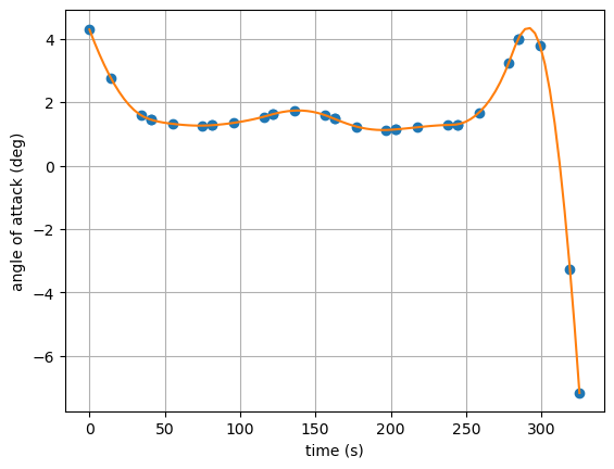
Both the simulate method and the interp method can provide more dense output. The difference is that simulate is effectively finding a different solution for the states, by starting from the initial values and propagating the ODE forward in time using the interpolated control splines as inputs. The interp method is making some assumptions about the interpolation (for instance, cubic interpolation in this case), so it may not be a perfectly accurate representation of the underlying interpolating polynomials.