Segments of Phases#
Things you’ll learn through this example
What are segments?
How does the number and order of segments affect the solution?
How to use the Dymos run_problem function to find the right number of segments automatically.
What are segments?#
In the previous section we showed a converged trajectory that didn’t really match the state propagation found using Scipy’s variable step solve_ivp method.
import openmdao.api as om
import dymos as dm
import matplotlib.pyplot as plt

from dymos.examples.oscillator.oscillator_ode import OscillatorODE

# Instantiate an OpenMDAO Problem instance.
prob = om.Problem()

# Instantiate a Dymos Trajectory and add it to the Problem model.
traj = dm.Trajectory()
prob.model.add_subsystem('traj', traj)

# Instantiate a Phase and add it to the Trajectory.
# Here the transcription is necessary but not particularly relevant.
phase = dm.Phase(ode_class=OscillatorODE, transcription=dm.Radau(num_segments=4))
traj.add_phase('phase0', phase)

# Tell Dymos the states to be propagated using the given ODE.
phase.add_state('v', rate_source='v_dot', targets=['v'], units='m/s')
phase.add_state('x', rate_source='v', targets=['x'], units='m')

# The spring constant, damping coefficient, and mass are inputs to the system
# that are constant throughout the phase.
phase.add_parameter('k', units='N/m', targets=['k'])
phase.add_parameter('c', units='N*s/m', targets=['c'])
phase.add_parameter('m', units='kg', targets=['m'])

# Setup the OpenMDAO problem
prob.setup()

# Assign values to the times and states
phase.set_time_val(0.0, 15.0)
phase.set_state_val('x', 10.0)
phase.set_state_val('v', 0.0)
phase.set_parameter_val('k', 1.0)
phase.set_parameter_val('c', 0.5)
phase.set_parameter_val('m', 1.0)

# Perform a single execution of the model (executing the model is required before simulation).
prob.run_model()

# Perform an explicit simulation of our ODE from the initial conditions.
sim_out = traj.simulate(times_per_seg=50)

# Plot the state values obtained from the phase timeseries objects in the simulation output.
t_sol = prob.get_val('traj.phase0.timeseries.time')
t_sim = sim_out.get_val('traj.phase0.timeseries.time')

states = ['x', 'v']
fig, axes = plt.subplots(len(states), 1)
for i, state in enumerate(states):
    sol = axes[i].plot(t_sol, prob.get_val(f'traj.phase0.timeseries.{state}'), 'o')
    sim = axes[i].plot(t_sim, sim_out.get_val(f'traj.phase0.timeseries.{state}'), '-')
    axes[i].set_ylabel(state)
axes[-1].set_xlabel('time (s)')
fig.legend((sol[0], sim[0]), ('solution', 'simulation'), loc='lower right', ncol=2)
plt.tight_layout()
plt.show()
Simulating trajectory traj
Done simulating trajectory traj
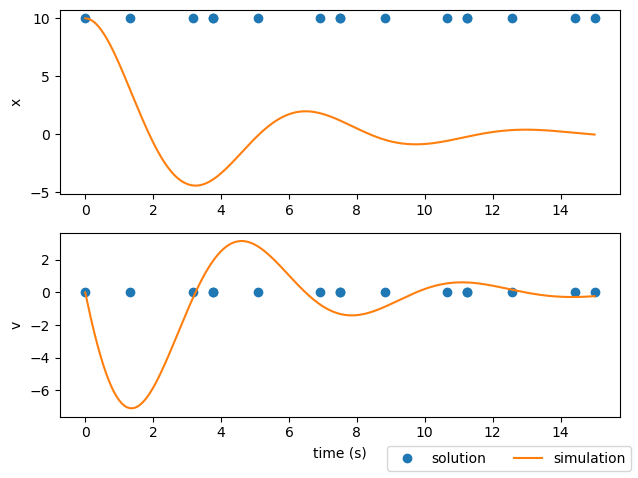
Why does this happen? The implicit collocation techniques used by Dymos (the Radau Pseudospectral Method and Legendre-Gauss-Lobatto collocation) work by discretizing a continuous function (the state time-history) into a series of discrete points. It does this by breaking the time domain of each phase into multiple polynomial segments. On each segment, each state is treated as a continuous polynomial of some given order. In Dymos, segments must have an order of at least 3. That is also the default order for segments.
How does the number and order of segments affect the solution?#
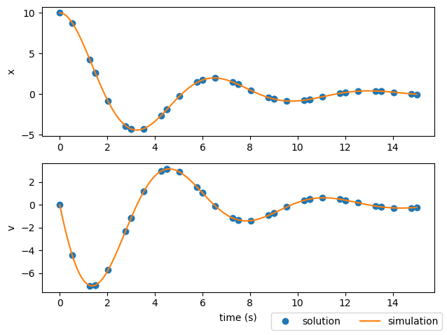
Obviously, a single third-order polynomial won’t be able to fit highly oscillatory behavior. In this case, our guess of using four segments (equally spaced) in the phase wasn’t quite sufficient. Let’s try increasing that number to ten third-order segments.
import openmdao.api as om
import dymos as dm
import matplotlib.pyplot as plt

from dymos.examples.oscillator.oscillator_ode import OscillatorODE

# Instantiate an OpenMDAO Problem instance.
prob = om.Problem()

# We need an optimization driver.  To solve this simple problem ScipyOptimizerDriver will work.
prob.driver = om.ScipyOptimizeDriver()

# Instantiate a Dymos Trajectory and add it to the Problem model.
traj = dm.Trajectory()
prob.model.add_subsystem('traj', traj)

# Instantiate a Phase and add it to the Trajectory.
phase = dm.Phase(ode_class=OscillatorODE, transcription=dm.Radau(num_segments=10))
traj.add_phase('phase0', phase)

# Tell Dymos that the duration of the phase is bounded.
phase.set_time_options(fix_initial=True, fix_duration=True)

# Tell Dymos the states to be propagated using the given ODE.
phase.add_state('x', fix_initial=True, rate_source='v', targets=['x'], units='m')
phase.add_state('v', fix_initial=True, rate_source='v_dot', targets=['v'], units='m/s')

# The spring constant, damping coefficient, and mass are inputs to the system that
# are constant throughout the phase.
phase.add_parameter('k', units='N/m', targets=['k'])
phase.add_parameter('c', units='N*s/m', targets=['c'])
phase.add_parameter('m', units='kg', targets=['m'])

# Since we're using an optimization driver, an objective is required.  We'll minimize
# the final time in this case.
phase.add_objective('time', loc='final')

# Setup the OpenMDAO problem
prob.setup()

# Assign values to the times and states
phase.set_time_val(0.0, 15.0)
phase.set_state_val('x', 10.0)
phase.set_state_val('v', 0.0)
phase.set_parameter_val('k', 1.0)
phase.set_parameter_val('c', 0.5)
phase.set_parameter_val('m', 1.0)

# Now we're using the optimization driver to iteratively run the model and vary the
# phase duration until the final y value is 0.
prob.run_driver()

# Perform an explicit simulation of our ODE from the initial conditions.
sim_out = traj.simulate(times_per_seg=50)

# Plot the state values obtained from the phase timeseries objects in the simulation output.
t_sol = prob.get_val('traj.phase0.timeseries.time')
t_sim = sim_out.get_val('traj.phase0.timeseries.time')

states = ['x', 'v']
fig, axes = plt.subplots(len(states), 1)
for i, state in enumerate(states):
    sol = axes[i].plot(t_sol, prob.get_val(f'traj.phase0.timeseries.{state}'), 'o')
    sim = axes[i].plot(t_sim, sim_out.get_val(f'traj.phase0.timeseries.{state}'), '-')
    axes[i].set_ylabel(state)
axes[-1].set_xlabel('time (s)')
fig.legend((sol[0], sim[0]), ('solution', 'simulation'), loc='lower right', ncol=2)
plt.tight_layout()
plt.show()
/home/runner/work/dymos/dymos/.openmdao-pixi/.pixi/envs/dev/lib/python3.13/site-packages/openmdao/core/driver.py:1276: DriverWarning:ScipyOptimizeDriver: objective(s) ['traj.phase0.t'] do not depend on any design variables. Please check your problem formulation.
/home/runner/work/dymos/dymos/.openmdao-pixi/.pixi/envs/dev/lib/python3.13/site-packages/openmdao/core/total_jac.py:1670: DerivativesWarning:The following constraints or objectives cannot be impacted by the design variables of the problem at the current design point:
  traj.phase0.t, inds=[39]
Optimization terminated successfully    (Exit mode 0)
            Current function value: 15.0
            Iterations: 1
            Function evaluations: 2
            Gradient evaluations: 1
Optimization Complete
-----------------------------------

Simulating trajectory traj
Done simulating trajectory traj
Alternatively, we could stick with 4 segments but give each a higher order (7 in this case).
import openmdao.api as om
import dymos as dm
import matplotlib.pyplot as plt

from dymos.examples.oscillator.oscillator_ode import OscillatorODE

# Instantiate an OpenMDAO Problem instance.
prob = om.Problem()

# We need an optimization driver.  To solve this simple problem ScipyOptimizerDriver will work.
prob.driver = om.ScipyOptimizeDriver()

# Instantiate a Dymos Trajectory and add it to the Problem model.
traj = dm.Trajectory()
prob.model.add_subsystem('traj', traj)

# Instantiate a Phase and add it to the Trajectory.
phase = dm.Phase(ode_class=OscillatorODE, transcription=dm.Radau(num_segments=4, order=7))
traj.add_phase('phase0', phase)

# Tell Dymos that the duration of the phase is bounded.
phase.set_time_options(fix_initial=True, fix_duration=True)

# Tell Dymos the states to be propagated using the given ODE.
phase.add_state('x', fix_initial=True, rate_source='v', targets=['x'], units='m')
phase.add_state('v', fix_initial=True, rate_source='v_dot', targets=['v'], units='m/s')

# The spring constant, damping coefficient, and mass are inputs to the system that are
# constant throughout the phase.
phase.add_parameter('k', units='N/m', targets=['k'])
phase.add_parameter('c', units='N*s/m', targets=['c'])
phase.add_parameter('m', units='kg', targets=['m'])

# Since we're using an optimization driver, an objective is required.  We'll minimize
# the final time in this case.
phase.add_objective('time', loc='final')

# Setup the OpenMDAO problem
prob.setup()

# Assign values to the times and states
phase.set_time_val(0.0, 15.0)
phase.set_state_val('x', 10.0)
phase.set_state_val('v', 0.0)
phase.set_parameter_val('k', 1.0)
phase.set_parameter_val('c', 0.5)
phase.set_parameter_val('m', 1.0)

# Now we're using the optimization driver to iteratively run the model and vary the
# phase duration until the final y value is 0.
prob.run_driver()

# Perform an explicit simulation of our ODE from the initial conditions.
sim_out = traj.simulate(times_per_seg=50)

# Plot the state values obtained from the phase timeseries objects in the simulation output.
t_sol = prob.get_val('traj.phase0.timeseries.time')
t_sim = sim_out.get_val('traj.phase0.timeseries.time')

states = ['x', 'v']
fig, axes = plt.subplots(len(states), 1)
for i, state in enumerate(states):
    sol = axes[i].plot(t_sol, prob.get_val(f'traj.phase0.timeseries.{state}'), 'o')
    sim = axes[i].plot(t_sim, sim_out.get_val(f'traj.phase0.timeseries.{state}'), '-')
    axes[i].set_ylabel(state)
axes[-1].set_xlabel('time (s)')
fig.legend((sol[0], sim[0]), ('solution', 'simulation'), loc='lower right', ncol=2)
plt.tight_layout()
plt.show()
/home/runner/work/dymos/dymos/.openmdao-pixi/.pixi/envs/dev/lib/python3.13/site-packages/openmdao/core/driver.py:1276: DriverWarning:ScipyOptimizeDriver: objective(s) ['traj.phase0.t'] do not depend on any design variables. Please check your problem formulation.
/home/runner/work/dymos/dymos/.openmdao-pixi/.pixi/envs/dev/lib/python3.13/site-packages/openmdao/core/total_jac.py:1670: DerivativesWarning:The following constraints or objectives cannot be impacted by the design variables of the problem at the current design point:
  traj.phase0.t, inds=[31]
Optimization terminated successfully    (Exit mode 0)
            Current function value: 15.0
            Iterations: 1
            Function evaluations: 2
            Gradient evaluations: 1
Optimization Complete
-----------------------------------

Simulating trajectory traj
Done simulating trajectory traj
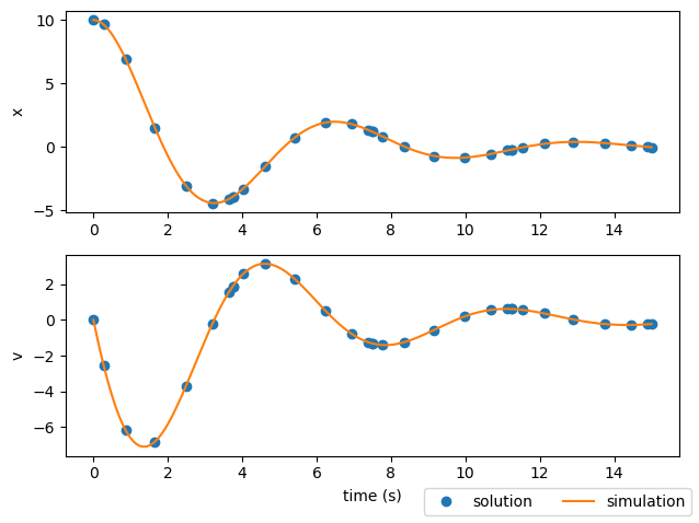
In both these cases, we obtained a better match of the dynamics using either more segments or higher-order segments. This gives the state interpolating polynomials enough freedom to more accurately match the true behavior of the system. Increasing the number of segments and increasing the segment orders both increase the number of discrete points, and thus slow down the solution a bit. Theres a balance to be found between using enough discretization points to get an accurate solution, and slowing down the analysis due to having an overabundance of points. In general, using a high number of low-order segments is preferable to using fewer high-order segments because it makes the constraint jacobian more sparse.
In addition to the number and order of the segments, the user can also provide the transcription the argument segment_ends. If None, the segments are equally distributed in time throughout the phase. Otherwise, segment_ends should be a monotonically increasing sequence of length num_segments + 1.
Each element in the sequence provides the location of a segment boundary in the phase.
The items in segment_ends are normalized by Dymos, so feel free to provide them in whatever scale makes sense.
That is, segment_ends=[0, 1, 2, 5] is equivalent to segment_ends=[10, 20, 30, 60].
Letting Dymos automatically find the right segmentation of the phase#
Manually tweaking the “grid” (the number of segments, their order, and relative spacing) isn’t ideal. In reality, another nested level of iteration is required:
Problem.run_model()evaluates the model and computes constraints and objectives based on the current design variables.Problem.run_driver()iteratively callsProblem.run_model()while varying the design variables in order to find a feasible, optimal design point.Some “outer” function iterates on
run_driver(), varying the grid until a satisfactory accuracy is achieved.
This third level is filled by the role of automated grid refinement via the dymos.run_problem. In the next section, we’ll learn how to use automated grid refinement in Dymos.