The Brachistochrone#
Things you’ll learn through this example
How to define a basic Dymos ODE system.
How to test the partials of your ODE system.
Adding a Trajectory object with a single Phase to an OpenMDAO Problem.
Imposing boundary conditions on states with simple bounds via
fix_initialandfix_final.Using the Phase.interpolate` method to set a linear guess for state and control values across the Phase.
Checking the validity of the result through explicit simulation via the
Trajectory.simulatemethod.
The brachistochrone is one of the most well-known optimal control problems. It was originally posed as a challenge by Johann Bernoulli.
The brachistochrone problem
Given two points A and B in a vertical plane, find the path AMB down which a movable point M must by virtue of its weight fall from A to B in the shortest possible time.
Johann Bernoulli, Acta Eruditorum, June 1696
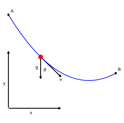
We seek to find the optimal shape of a wire between two points (A and B) such that a bead sliding without friction along the wire moves from point A to point B in minimum time.
State variables#
In this implementation, three state variables are used to define the configuration of the system at any given instant in time.
x: The horizontal position of the particle at an instant in time.
y: The vertical position of the particle at an instant in time.
v: The speed of the particle at an instant in time.
System dynamics#
From the free-body diagram above, the evolution of the state variables is given by the following ordinary differential equations (ODE).
Control variables#
This system has a single control variable.
\(\theta\): The angle between the gravity vector and the tangent to the curve at the current instant in time.
The initial and final conditions#
In this case, starting point A is given as (0, 10). The point moving along the curve will begin there with zero initial velocity.
The initial conditions are:
The end point B is given as (10, 5). The point will end there, but the velocity at that point is not constrained.
The final conditions are:
Defining the ODE as an OpenMDAO System#
In Dymos, the ODE is an OpenMDAO System (a Component, or a Group of components). The following ExplicitComponent computes the state rates for the brachistochrone problem.
More detail on the workings of an ExplicitComponent can be found in the OpenMDAO documentation. In summary:
initialize: Called at setup, and used to define options for the component. ALL Dymos ODE components should have the property
num_nodes, which defines the number of points at which the outputs are simultaneously computed.setup: Used to add inputs and outputs to the component, and declare which outputs (and indices of outputs) are dependent on each of the inputs.
compute: Used to compute the outputs, given the inputs.
compute_partials: Used to compute the derivatives of the outputs w.r.t. each of the inputs analytically. This method may be omitted if finite difference or complex-step approximations are used, though analytic is recommended.
import numpy as np
import openmdao.api as om


class BrachistochroneODE(om.ExplicitComponent):

    def initialize(self):
        self.options.declare('num_nodes', types=int)
        self.options.declare('static_gravity', types=(bool,), default=False,
                             desc='If True, treat gravity as a static (scalar) input, rather than '
                                  'having different values at each node.')

    def setup(self):
        nn = self.options['num_nodes']

        # Inputs
        self.add_input('v', val=np.zeros(nn), desc='velocity', units='m/s')

        if self.options['static_gravity']:
            self.add_input('g', val=9.80665, desc='grav. acceleration', units='m/s/s',
                           tags=['dymos.static_target'])
        else:
            self.add_input('g', val=9.80665 * np.ones(nn), desc='grav. acceleration', units='m/s/s')

        self.add_input('theta', val=np.ones(nn), desc='angle of wire', units='rad')

        self.add_output('xdot', val=np.zeros(nn), desc='velocity component in x', units='m/s',
                        tags=['dymos.state_rate_source:x', 'dymos.state_units:m'])

        self.add_output('ydot', val=np.zeros(nn), desc='velocity component in y', units='m/s',
                        tags=['dymos.state_rate_source:y', 'dymos.state_units:m'])

        self.add_output('vdot', val=np.zeros(nn), desc='acceleration magnitude', units='m/s**2',
                        tags=['dymos.state_rate_source:v', 'dymos.state_units:m/s'])

        self.add_output('check', val=np.zeros(nn), desc='check solution: v/sin(theta) = constant',
                        units='m/s')

        # Setup partials
        arange = np.arange(self.options['num_nodes'])
        self.declare_partials(of='vdot', wrt='theta', rows=arange, cols=arange)

        self.declare_partials(of='xdot', wrt='v', rows=arange, cols=arange)
        self.declare_partials(of='xdot', wrt='theta', rows=arange, cols=arange)

        self.declare_partials(of='ydot', wrt='v', rows=arange, cols=arange)
        self.declare_partials(of='ydot', wrt='theta', rows=arange, cols=arange)

        self.declare_partials(of='check', wrt='v', rows=arange, cols=arange)
        self.declare_partials(of='check', wrt='theta', rows=arange, cols=arange)

        if self.options['static_gravity']:
            c = np.zeros(self.options['num_nodes'])
            self.declare_partials(of='vdot', wrt='g', rows=arange, cols=c)
        else:
            self.declare_partials(of='vdot', wrt='g', rows=arange, cols=arange)

    def compute(self, inputs, outputs):
        theta = inputs['theta']
        cos_theta = np.cos(theta)
        sin_theta = np.sin(theta)
        g = inputs['g']
        v = inputs['v']

        outputs['vdot'] = g * cos_theta
        outputs['xdot'] = v * sin_theta
        outputs['ydot'] = -v * cos_theta
        outputs['check'] = v / sin_theta

    def compute_partials(self, inputs, partials):
        theta = inputs['theta']
        cos_theta = np.cos(theta)
        sin_theta = np.sin(theta)
        g = inputs['g']
        v = inputs['v']

        partials['vdot', 'g'] = cos_theta
        partials['vdot', 'theta'] = -g * sin_theta

        partials['xdot', 'v'] = sin_theta
        partials['xdot', 'theta'] = v * cos_theta

        partials['ydot', 'v'] = -cos_theta
        partials['ydot', 'theta'] = v * sin_theta

        partials['check', 'v'] = 1 / sin_theta
        partials['check', 'theta'] = -v * cos_theta / sin_theta ** 2
“Things to note about the ODE system”
There is no input for the position states (\(x\) and \(y\)). The dynamics aren’t functions of these states, so they aren’t needed as inputs.
While \(g\) is an input to the system, since it will never change throughout the trajectory, it can be an option on the system. This way we don’t have to define any partials w.r.t. \(g\).
The output
checkis an auxiliary output, not a rate of the state variables. In this case, optimal control theory tells us thatcheckshould be constant throughout the trajectory, so it’s a useful output from the ODE.
Testing the ODE#
Now that the ODE system is defined, it is strongly recommended to test the analytic partials before using it in optimization.
If the partials are incorrect, then the optimization will almost certainly fail.
Fortunately, OpenMDAO makes testing derivatives easy with the check_partials method.
The assert_check_partials method in openmdao.utils.assert_utils can be used in test frameworks to verify the correctness of the partial derivatives in a model.
The following is a test method which creates a new OpenMDAO problem whose model contains the ODE class.
The problem is setup with the force_alloc_complex=True argument to enable complex-step approximation of the derivatives.
Complex step typically produces derivative approximations with an error on the order of 1.0E-16, as opposed to ~1.0E-6 for forward finite difference approximations.
import numpy as np
import openmdao.api as om

num_nodes = 5

p = om.Problem(model=om.Group())

ivc = p.model.add_subsystem('vars', om.IndepVarComp())
ivc.add_output('v', shape=(num_nodes,), units='m/s')
ivc.add_output('theta', shape=(num_nodes,), units='deg')

p.model.add_subsystem('ode', BrachistochroneODE(num_nodes=num_nodes))

p.model.connect('vars.v', 'ode.v')
p.model.connect('vars.theta', 'ode.theta')

p.setup(force_alloc_complex=True)

p.set_val('vars.v', 10*np.random.random(num_nodes))
p.set_val('vars.theta', 10*np.random.uniform(1, 179, num_nodes))

p.run_model()
cpd = p.check_partials(method='cs', compact_print=True)
------------------------------------------------------------------------
Component: BrachistochroneODE 'ode'
------------------------------------------------------------------------

+---------------+----------------+---------------------+-------------------+------------------------+------------+
| 'of' variable | 'wrt' variable | calc val @ max viol | fd val @ max viol | (calc-fd) - (a + r*fd) | error desc |
+===============+================+=====================+===================+========================+============+
| check         | g              |        0.000000e+00 |     -0.000000e+00 |         (0.000000e+00) |            |
+---------------+----------------+---------------------+-------------------+------------------------+------------+
| check         | theta          |        0.000000e+00 |      0.000000e+00 |         (0.000000e+00) |            |
+---------------+----------------+---------------------+-------------------+------------------------+------------+
| check         | v              |        0.000000e+00 |      0.000000e+00 |         (0.000000e+00) |            |
+---------------+----------------+---------------------+-------------------+------------------------+------------+
| vdot          | g              |        0.000000e+00 |      0.000000e+00 |         (0.000000e+00) |            |
+---------------+----------------+---------------------+-------------------+------------------------+------------+
| vdot          | theta          |        0.000000e+00 |      0.000000e+00 |         (0.000000e+00) |            |
+---------------+----------------+---------------------+-------------------+------------------------+------------+
| vdot          | v              |        0.000000e+00 |      0.000000e+00 |         (0.000000e+00) |            |
+---------------+----------------+---------------------+-------------------+------------------------+------------+
| xdot          | g              |        0.000000e+00 |     -0.000000e+00 |         (0.000000e+00) |            |
+---------------+----------------+---------------------+-------------------+------------------------+------------+
| xdot          | theta          |        0.000000e+00 |      0.000000e+00 |         (0.000000e+00) |            |
+---------------+----------------+---------------------+-------------------+------------------------+------------+
| xdot          | v              |        0.000000e+00 |      0.000000e+00 |         (0.000000e+00) |            |
+---------------+----------------+---------------------+-------------------+------------------------+------------+
| ydot          | g              |        0.000000e+00 |      0.000000e+00 |         (0.000000e+00) |            |
+---------------+----------------+---------------------+-------------------+------------------------+------------+
| ydot          | theta          |        0.000000e+00 |      0.000000e+00 |         (0.000000e+00) |            |
+---------------+----------------+---------------------+-------------------+------------------------+------------+
| ydot          | v              |        0.000000e+00 |      0.000000e+00 |         (0.000000e+00) |            |
+---------------+----------------+---------------------+-------------------+------------------------+------------+
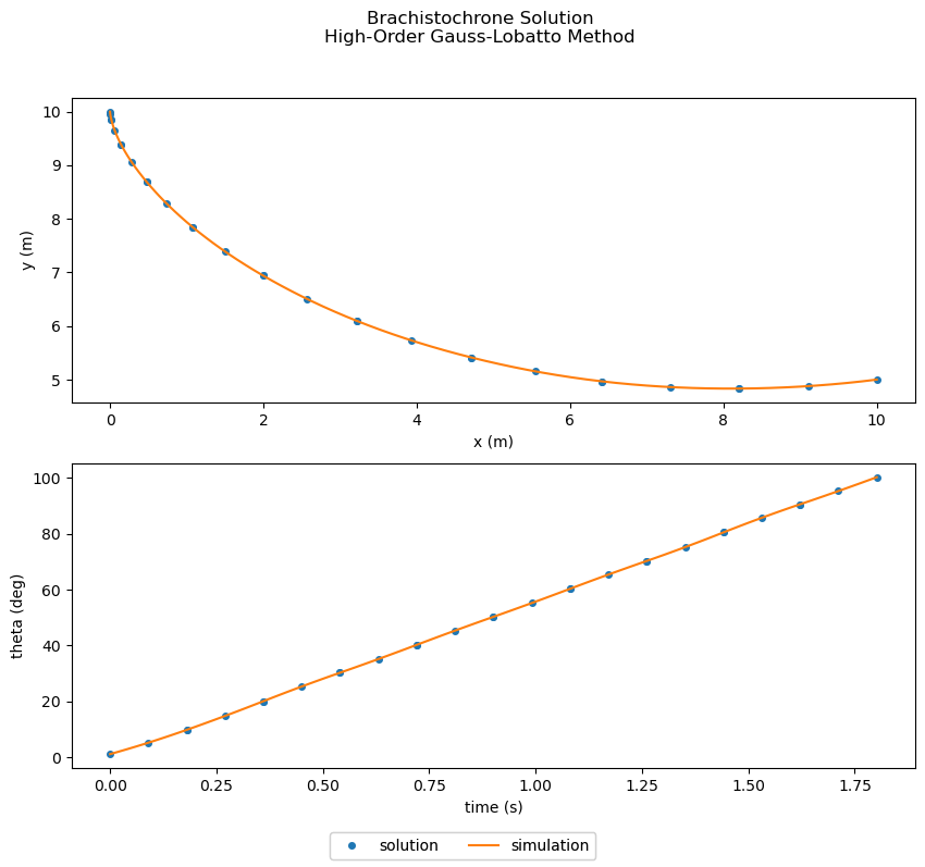
Solving the problem with Legendre-Gauss-Lobatto collocation in Dymos#
The following script fully defines the brachistochrone problem with Dymos and solves it. In this section we’ll walk through each step.
import openmdao.api as om
import dymos as dm
from dymos.examples.plotting import plot_results
from dymos.examples.brachistochrone import BrachistochroneODE
import matplotlib.pyplot as plt

#
# Initialize the Problem and the optimization driver
#
p = om.Problem(model=om.Group())
p.driver = om.ScipyOptimizeDriver()
p.driver.declare_coloring()

#
# Create a trajectory and add a phase to it
#
traj = p.model.add_subsystem('traj', dm.Trajectory())

phase = traj.add_phase('phase0',
                       dm.Phase(ode_class=BrachistochroneODE,
                                transcription=dm.GaussLobatto(num_segments=10)))

#
# Set the variables
#
phase.set_time_options(fix_initial=True, duration_bounds=(.5, 10))

phase.add_state('x', fix_initial=True, fix_final=True)

phase.add_state('y', fix_initial=True, fix_final=True)

phase.add_state('v', fix_initial=True, fix_final=False)

phase.add_control('theta', continuity=True, rate_continuity=True,
                  units='deg', lower=0.01, upper=179.9)

phase.add_parameter('g', units='m/s**2', val=9.80665)

#
# Minimize time at the end of the phase
#
phase.add_objective('time', loc='final', scaler=10)

p.model.linear_solver = om.DirectSolver()

#
# Setup the Problem
#
p.setup()

#
# Set the initial values
#
phase.set_time_val(initial=0.0, duration=2.0)
phase.set_state_val('x', [0, 10])
phase.set_state_val('y', [10, 5])
phase.set_state_val('v', [0, 9.9])
phase.set_control_val('theta', [5, 100.5])

#
# Solve for the optimal trajectory
#
dm.run_problem(p)

# Check the results
print(p.get_val('traj.phase0.timeseries.time')[-1])
Jacobian shape: (40, 50)  (13.40% nonzero)
FWD solves: 8   REV solves: 0
Total colors vs. total size: 8 vs 50  (84.00% improvement)

Sparsity computed using tolerance: 1e-25.
Dense total jacobian for Problem 'problem2' was computed 3 times.
Time to compute sparsity:   0.0156 sec
Time to compute coloring:   0.0334 sec
Memory to compute coloring:   0.2891 MB
Coloring created on: 2026-05-13 14:54:43
/home/runner/work/dymos/dymos/.openmdao-pixi/.pixi/envs/dev/lib/python3.13/site-packages/openmdao/utils/relevance.py:1234: OpenMDAOWarning:The top level group has a nonlinear solver that computes gradients, so the entire model will be included in the optimization iteration.
Optimization terminated successfully    (Exit mode 0)
            Current function value: 18.016167304638337
            Iterations: 24
            Function evaluations: 24
            Gradient evaluations: 24
Optimization Complete
-----------------------------------
[1.80161673]
# Generate the explicitly simulated trajectory
exp_out = traj.simulate()

plot_results([('traj.phase0.timeseries.x', 'traj.phase0.timeseries.y',
               'x (m)', 'y (m)'),
              ('traj.phase0.timeseries.time', 'traj.phase0.timeseries.theta',
               'time (s)', 'theta (deg)')],
             title='Brachistochrone Solution\nHigh-Order Gauss-Lobatto Method',
             p_sol=p, p_sim=exp_out)

plt.show()
Simulating trajectory traj
Done simulating trajectory traj
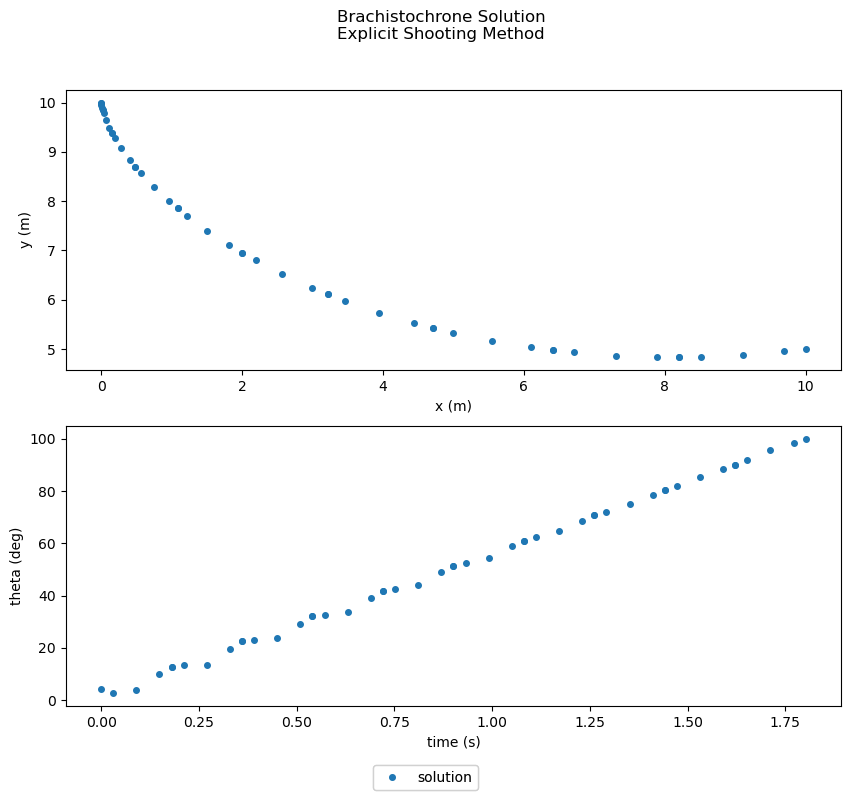
Solving the problem with single shooting in Dymos#
The following script fully defines the brachistochrone problem with Dymos and solves it using a single explicit shooting method.
The code is nearly identical to that using the collocation approach.
Key differences are shown when defining the transcription, specifying how to constrain the final state values of x and y states, and providing initial guesses for all states.
The ExplicitShooting transcription may accept a Grid objects: the grid dictates where the controls are defined, and the nodes one which outputs are provided in the phase timeseries.
If one uses the standard arguments to other transcriptions (num_segments, order, etc.), then dymos will assume the use of a GaussLobattoGrid distribution to define the nodes for ExplicitShooting.
Since the order specification is somewhat ambiguous (especially for explicit shooting where it doesn’t impact the behavior of the state), the Grid objects use nodes_per_seg instead of order.
import openmdao.api as om
import dymos as dm
from dymos.examples.plotting import plot_results
from dymos.examples.brachistochrone import BrachistochroneODE
import matplotlib.pyplot as plt

#
# Initialize the Problem and the optimization driver
#
p = om.Problem(model=om.Group())
p.driver = om.ScipyOptimizeDriver()

# We'll try to use coloring, but OpenMDAO will tell us that it provides no benefit.
p.driver.declare_coloring()

#
# Create a trajectory and add a phase to it
#
traj = p.model.add_subsystem('traj', dm.Trajectory())

grid = dm.GaussLobattoGrid(num_segments=10, nodes_per_seg=5)

phase = traj.add_phase('phase0',
                       dm.Phase(ode_class=BrachistochroneODE,
                                transcription=dm.ExplicitShooting(grid=grid)))

#
# Set the variables
#
phase.set_time_options(fix_initial=True, duration_bounds=(.5, 10))

# Note, we cannot use fix_final=True with the shooting method
# because the final value of the states are
# not design variables in the transcribed optimization problem.
phase.add_state('x', fix_initial=True)

phase.add_state('y', fix_initial=True)

phase.add_state('v', fix_initial=True)

phase.add_control('theta', continuity=True, rate_continuity=True,
                  units='deg', lower=0.01, upper=179.9)

phase.add_parameter('g', units='m/s**2', val=9.80665)

#
# Minimize time at the end of the phase
#
phase.add_objective('time', loc='final', scaler=10)

#
# Add boundary constraints for x and y since we could not use `fix_final=True`
#
phase.add_boundary_constraint('x', loc='final', equals=10)
phase.add_boundary_constraint('y', loc='final', equals=5)

p.model.linear_solver = om.DirectSolver()

#
# Setup the Problem
#
p.setup()

#
# Set the initial values
#
phase.set_time_val(initial=0.0, duration=2.0)
phase.set_state_val('x', [0, 10])
phase.set_state_val('y', [10, 5])
phase.set_state_val('v', [0, 9.9])
phase.set_control_val('theta', [5, 100.5])

#
# Solve for the optimal trajectory
#
dm.run_problem(p)

# Check the results
print(p.get_val('traj.phase0.timeseries.time')[-1])
/home/runner/work/dymos/dymos/.openmdao-pixi/.pixi/envs/dev/lib/python3.13/site-packages/openmdao/utils/relevance.py:1234: OpenMDAOWarning:The top level group has a nonlinear solver that computes gradients, so the entire model will be included in the optimization iteration.
No coloring was computed successfully.
/home/runner/work/dymos/dymos/.openmdao-pixi/.pixi/envs/dev/lib/python3.13/site-packages/openmdao/utils/coloring.py:447: DerivativesWarning:Coloring was deactivated. Improvement of 0.0% was less than min allowed (5.0%).
Optimization terminated successfully    (Exit mode 0)
            Current function value: 18.01852077656255
            Iterations: 11
            Function evaluations: 12
            Gradient evaluations: 11
Optimization Complete
-----------------------------------
/home/runner/work/dymos/dymos/.openmdao-pixi/.pixi/envs/dev/lib/python3.13/site-packages/openmdao/visualization/opt_report/opt_report.py:611: UserWarning: Attempting to set identical low and high ylims makes transformation singular; automatically expanding.
  ax.set_ylim([ymin_plot, ymax_plot])
[1.80185208]
plot_results([('traj.phase0.timeseries.x', 'traj.phase0.timeseries.y',
               'x (m)', 'y (m)'),
              ('traj.phase0.timeseries.time', 'traj.phase0.timeseries.theta',
               'time (s)', 'theta (deg)')],
             title='Brachistochrone Solution\nExplicit Shooting Method',
             p_sol=p)

plt.show()