The Bryson-Denham Problem

The Bryson-Denham Problem#

The Bryson-Denham problem is a variation of the double integrator problem [BH75]. It can be stated as:

Minimize the control effort required to reverse the direction of motion of a frictionless sliding block such that the reversal happens with some limited amount of displacement.

State and control variables#

This system has two state variables, the position (\(x\)) and velocity (\(v\)) of the sliding block.

This system has a single control variable (\(u\)), the acceleration of the block.

The dynamics of the system are governed by

(27)#\[\begin{align} \dot{x} &= v \\ \dot{v} &= u \end{align}\]

Problem Definition#

We seek to minimize the time required to exit the well in the positive direction.

(28)#\[\begin{align} \mathrm{Minimize} \, J &= 0.5 \int_0^1 u^2 dt \end{align}\]

Subject to the initial conditions

(29)#\[\begin{align} x_0 &= 0.0 \\ v_0 &= 1.0 \end{align}\]

and the terminal constraints

(30)#\[\begin{align} x_f &= 0.0 \\ v_f &= -1.0 \end{align}\]

In addition, \(x\) is constrained to remain below a displacement of 1/9.

(31)#\[\begin{align} x &\le 1/9 \end{align}\]

Dealing with integral costs in Dymos#

In classic optimal control, the objective is often broken into the terminal component (the Mayer term) and the integral component (the Lagrange term). Dymos does not distinguish between the two. In this case, since the objective \(J\) is an integrated quantity, we add a term to the ODE

(32)#\[\begin{align} \dot{J} &= 0.5 u^2 \end{align}\]

Defining the ODE#

The following code implements the equations of motion for the mountain car problem. Since the rate of \(x\) is given by another state (\(v\)), and the rate of \(v\) is given by a control (\(u\)), there is no need to compute their rates in the ODE. Dymos can pull their values from those other states and controls. The ODE, therefore, only needs to compute the rate of change of \(J\).

A few things to note:

By providing the tag dymos.state_rate_source:{name}, we’re letting Dymos know what states need to be integrated, there’s no need to specify a rate source when using this ODE in our Phase.
Pairing the above tag with dymos.state_units:{units} means we don’t have to specify units when setting properties for the state in our run script.

import numpy as np
import openmdao.api as om


class BrysonDenhamODE(om.ExplicitComponent):
    
    def initialize(self):
        self.options.declare('num_nodes', types=int)
        
    def setup(self):
        nn = self.options['num_nodes']
        
        self.add_input('x', shape=(nn,), units='m')
        self.add_input('v', shape=(nn,), units='m/s')
        self.add_input('u', shape=(nn,), units='m/s**2')
        
        self.add_output('J_dot', shape=(nn,), units='m**2/s**4',
                        tags=['dymos.state_rate_source:J',
                              'dymos.state_units:m**2/s**3'])
        
        ar = np.arange(nn, dtype=int)
        
        self.declare_partials(of='J_dot', wrt='u', rows=ar, cols=ar)

    def compute(self, inputs, outputs):
        u = inputs['u']
        outputs['J_dot'] = 0.5 * u**2

    def compute_partials(self, inputs, partials):
        partials['J_dot', 'u'] = inputs['u']
        

Solving the Bryson-Denham problem with Dymos#

The following script solves the minimum-time mountain car problem with Dymos. This problem is pretty trivial and can be solved using the SLSQP optimizer in scipy.

To begin, import the packages we require:

import dymos as dm
import matplotlib.pyplot as plt

We then instantiate an OpenMDAO problem and set the optimizer and its options.

The call to declare_coloring tells the optimizer to attempt to find a sparsity pattern that minimizes the work required to compute the derivatives across the model.

SLSQP does not internally use this sparsity information to reduce memory and improve performance as some other optimizers do, but the performance due to the increased efficiency in computing derivatives still makes it worthwhile.

#
# Initialize the Problem and the optimization driver
#
p = om.Problem()
               
p.driver = om.ScipyOptimizeDriver()
p.driver.declare_coloring()

Next, we add a Dymos Trajectory group to the problem’s model and add a phase to it.

In this case we’re using the Radau pseudospectral transcription to solve the problem.

#
# Create a trajectory and add a phase to it
#
traj = p.model.add_subsystem('traj', dm.Trajectory())
tx = transcription=dm.Radau(num_segments=24)
phase = traj.add_phase('phase0', dm.Phase(ode_class=BrysonDenhamODE, transcription=tx))

At this point, we set the options on the main variables used in a Dymos phase.

In addition to time, we have three states (x, v, and J) and a single control (u).

Here we use bounds on the states themselves to constrain the initial and final value of x and v, and the initial value of J. From an optimization perspective, this means that we are removing the first and last values in the state histories of \(x\) and \(v\) from the vector of design variables. Their initial and final values will remain unchanged throughout the optimization process.

On the other hand, we could specify fix_initial=False, fix_final=False for these values, and Dymos would be free to change them. We would then need to put a boundary constraint in place to enforce their final values. Feel free to experiment with different ways of enforcing the boundary constraints on this problem and see how it affects performance.

The scaler values (ref) are all set to 1 here.

Bounds on time duration are guesses, and the bounds on the states and controls come from the implementation in the references.

Also, we don’t need to specify targets for any of the variables here because their names are the targets in the top-level of the model. The rate source and units for the states are obtained from the tags in the ODE component we previously defined.

#
# Set the variables
#
phase.set_time_options(fix_initial=True, fix_duration=True)

phase.add_state('x', fix_initial=True, fix_final=True, rate_source='v')
phase.add_state('v', fix_initial=True, fix_final=True, rate_source='u')
phase.add_state('J', fix_initial=True, fix_final=False) # Rate source obtained from tags on the ODE outputs
phase.add_control('u', continuity=True, rate_continuity=False)

#
# Minimize time at the end of the phase
#
phase.add_objective('J', loc='final', ref=1)
phase.add_path_constraint('x', upper=1/9)

#
# Setup the Problem
#
p.setup()

--- Constraint Report [traj] ---
    --- phase0 ---
        [path]     x <= 1.1111e-01  [m]

<openmdao.core.problem.Problem at 0x7f9549926770>

We then set the initial guesses for the variables in the problem and solve it.

We’re using the phase interp method to provide initial guesses for the states and controls. In this case, by giving it two values, it is linearly interpolating from the first value to the second value, and then returning the interpolated value at the input nodes for the given variable.

Finally, we use the dymos.run_problem method to execute the problem. This interface allows us to do some things that the standard OpenMDAO problem.run_driver interface does not. It will automatically record the final solution achieved by the optimizer in case named 'final' in a file called dymos_solution.db. By specifying simulate=True, it will automatically follow the solution with an explicit integration using scipy.solve_ivp. The results of the simulation are stored in a case named final in the file dymos_simulation.db. This explicit simulation demonstrates how the system evolved with the given controls, and serves as a check that we’re using a dense enough grid (enough segments and segments of sufficient order) to accurately represent the solution.

If those two solution didn’t agree reasonably well, we could rerun the problem with a more dense grid. Instead, we’re asking Dymos to automatically change the grid if necessary by specifying refine_method='ph'. This will attempt to repeatedly solve the problem and change the number of segments and segment orders until the solution is in reasonable agreement.

#
# Set the initial values
#
p['traj.phase0.t_initial'] = 0.0
p['traj.phase0.t_duration'] = 1.0

p.set_val('traj.phase0.states:x', phase.interp('x', ys=[0, 0]))
p.set_val('traj.phase0.states:v', phase.interp('v', ys=[1, -1]))
p.set_val('traj.phase0.states:J', phase.interp('J', ys=[0, 1]))
p.set_val('traj.phase0.controls:u', np.sin(phase.interp('u', ys=[0, 0])))

#
# Solve for the optimal trajectory
#
dm.run_problem(p, run_driver=True, simulate=True)

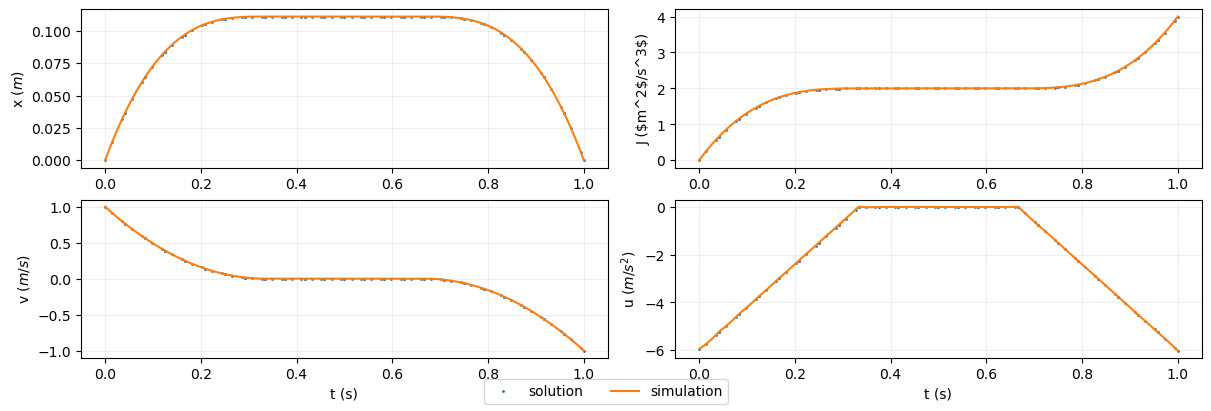
Plotting the solution#

The recommended practice is to obtain values from the recorded cases. While the problem object can also be queried for values, building plotting scripts that use the case recorder files as the data source means that the problem doesn’t need to be solved just to change a plot. Here we load values of various variables from the solution and simulation for use in the animation to follow.

sol = om.CaseReader('dymos_solution.db').get_case('final')
sim = om.CaseReader('dymos_simulation.db').get_case('final')

t = sol.get_val('traj.phase0.timeseries.time')
x = sol.get_val('traj.phase0.timeseries.x')
v = sol.get_val('traj.phase0.timeseries.v')
J = sol.get_val('traj.phase0.timeseries.J')
u = sol.get_val('traj.phase0.timeseries.u')
h = np.sin(3 * x) / 3

t_sim = sim.get_val('traj.phase0.timeseries.time')
x_sim = sim.get_val('traj.phase0.timeseries.x')
v_sim = sim.get_val('traj.phase0.timeseries.v')
J_sim = sim.get_val('traj.phase0.timeseries.J')
u_sim = sim.get_val('traj.phase0.timeseries.u')
h_sim = np.sin(3 * x_sim) / 3

fig = plt.figure(constrained_layout=True, figsize=(12, 4))
gs = fig.add_gridspec(2, 2)

x_ax = fig.add_subplot(gs[0, 0])
v_ax = fig.add_subplot(gs[1, 0])
J_ax = fig.add_subplot(gs[0, 1])
u_ax = fig.add_subplot(gs[1, 1])

x_ax.set_ylabel('x ($m$)')
v_ax.set_ylabel('v ($m/s$)')
J_ax.set_ylabel('J ($m^2$/s^3$)')
u_ax.set_ylabel('u ($m/s^2$)')
v_ax.set_xlabel('t (s)')
u_ax.set_xlabel('t (s)')

x_sol_handle, = x_ax.plot(t, x, 'o', ms=1)
v_ax.plot(t, v, 'o', ms=1)
J_ax.plot(t, J, 'o', ms=1)
u_ax.plot(t, u, 'o', ms=1)

x_sim_handle, = x_ax.plot(t_sim, x_sim, '-', ms=1)
v_ax.plot(t_sim, v_sim, '-', ms=1)
J_ax.plot(t_sim, J_sim, '-', ms=1)
u_ax.plot(t_sim, u_sim, '-', ms=1)

for ax in [x_ax, v_ax, J_ax, u_ax]:
    ax.grid(True, alpha=0.2)
    
plt.figlegend([x_sol_handle, x_sim_handle], ['solution', 'simulation'], ncol=2, loc='lower center');

../../_images/7593695aa4f804dc6c806ef005ca9e472dffefd6fa40e35ed0c0d0a54ac21f49.png

Animating the Solution#

The collapsed code cell below contains the code used to produce an animation of the mountain car solution using Matplotlib.

The green area represents the hilly terrain the car is traversing. The black circle is the center of the car, and the orange arrow is the applied control.

The applied control generally has the same sign as the velocity and is ‘bang-bang’, that is, it wants to be at its maximum possible magnitude. Interestingly, the sign of the control flips shortly before the sign of the velocity changes.

Show code cell source Hide code cell source

import matplotlib as mpl
from matplotlib import animation

BLOCK_SIZE = 0.02
X_EXTENTS = (-0.025, 0.175)

fig = plt.figure(constrained_layout=True, figsize=(12, 6))
gs = fig.add_gridspec(3, 2)

anim_ax = fig.add_subplot(gs[:, 0])
anim_ax.set_aspect('equal')

x_ax = fig.add_subplot(gs[0, 1:])
v_ax = fig.add_subplot(gs[1, 1:])
u_ax = fig.add_subplot(gs[2, 1:])

x_ax.set_ylabel('x')
v_ax.set_ylabel('v')
u_ax.set_ylabel('u')
u_ax.set_xlabel('t')

# set up the subplots as needed
anim_ax.set_xlim(X_EXTENTS);
y_extents = [-np.diff(X_EXTENTS) / 2, np.diff(X_EXTENTS) / 2]
anim_ax.set_ylim(y_extents);
anim_ax.set_xlabel('x');
anim_ax.set_yticks([])
time_text = anim_ax.text(0.05, 0.9, 't = 0.000 s', fontsize=16, transform=anim_ax.transAxes)

x_sol_line, = x_ax.plot(t, x, 'o', ms=1, label='solution', color='k')
v_ax.plot(t, v, 'o', ms=1, color='k')
u_ax.plot(t, u, 'o', ms=1, color='k')

x_sim_line, = x_ax.plot([], [], '-', linewidth=3, label='simulation', color='tab:blue')
v_sim_line, = v_ax.plot([], [], '-', linewidth=3, color='tab:red')
u_sim_line, = u_ax.plot([], [], '-', linewidth=3, color='tab:orange')

plt.figlegend(ncol=2, handles=[x_sol_line, x_sim_line], loc='upper center',
              bbox_to_anchor=(0.78,0.98))

x_ax.grid(alpha=0.2)
txt_x = x_ax.text(0.8, 0.1, f'x = {x_sim[0, 0]:6.3f}', horizontalalignment='left',
                  verticalalignment='center', transform=x_ax.transAxes)

v_ax.grid(alpha=0.2)
txt_v = v_ax.text(0.8, 0.1, f'v = {v_sim[0, 0]:6.3f}', horizontalalignment='left',
                  verticalalignment='center', transform=v_ax.transAxes)

u_ax.grid(alpha=0.2)
txt_u = u_ax.text(0.8, 0.1, f'u = {u_sim[0, 0]:6.3f}', horizontalalignment='left',
                  verticalalignment='center', transform=u_ax.transAxes)

x_terrain = np.linspace(-0.025, 0.175, 2);
h_terrain = 0 * x_terrain
terrain_line, = anim_ax.plot(x_terrain, h_terrain, '-', color='tab:gray', lw=2);
terrain = anim_ax.fill_between(x_terrain, h_terrain, h_terrain-1, color='tab:green');
wall = mpl.patches.Rectangle(xy=(1/9 + BLOCK_SIZE, 0), width=BLOCK_SIZE, height=3*BLOCK_SIZE, color='tab:gray')
anim_ax.add_patch(wall)
block = mpl.patches.Rectangle(xy=(0, 0), width=BLOCK_SIZE, height=BLOCK_SIZE, alpha=0.5)
anim_ax.add_patch(block)
v_vec = anim_ax.quiver(x_sim[0,0] + BLOCK_SIZE / 2, BLOCK_SIZE * 0.25, v_sim[0,0], [0], scale=10, angles='xy', color='tab:red')
u_vec = anim_ax.quiver(x_sim[0,0] + BLOCK_SIZE / 2, BLOCK_SIZE * 0.75, u_sim[0,0], [0], scale=50, angles='xy', color='tab:orange')

# See https://brushingupscience.com/2019/08/01/elaborate-matplotlib-animations/ for quiver animation

ANIM_DURATION = 3
PRE_PAUSE_DURATION = 1
POST_PAUSE_DURATION = 0.5
ANIM_FPS = 20

num_points = t_sim.size
num_frames = int(ANIM_DURATION * ANIM_FPS)
pre_pause_frames = int(PRE_PAUSE_DURATION * ANIM_FPS)
post_pause_frames = int(POST_PAUSE_DURATION * ANIM_FPS)

idx_from_frame_num = np.linspace(0, num_points-1, num_frames, dtype=int)

def drawframe(n):

    if n < pre_pause_frames:
        idx = 0
    elif n - pre_pause_frames >= idx_from_frame_num.size:
        idx = num_points - 1
    else:
        idx = idx_from_frame_num[n - pre_pause_frames]

    x = x_sim[idx]
    v = v_sim[idx]
    u = u_sim[idx]
    t = t_sim[idx]
    h = 0
    block.set_xy((x[0], h))
    
    v_vec.set_offsets((x[0] + BLOCK_SIZE/2, BLOCK_SIZE * 0.25))
    v_vec.set_UVC(v, 0)

    u_vec.set_offsets((x[0] + BLOCK_SIZE/2, BLOCK_SIZE * 0.75))
    u_vec.set_UVC(u, 0)

    x_sim_line.set_data(t_sim[:idx], x_sim[:idx])
    v_sim_line.set_data(t_sim[:idx], v_sim[:idx])
    u_sim_line.set_data(t_sim[:idx], u_sim[:idx])

    txt_x.set_text(f'x = {x[0]:6.3f}')
    txt_v.set_text(f'v = {v[0]:6.3f}')
    txt_u.set_text(f'u = {u[0]:6.3f}')
    
    time_text.set_text(f't = {t[0]:6.3f}')
    
    return block, u_vec, v_vec, x_sim_line, v_sim_line, u_sim_line, time_text

# # blit=True re-draws only the parts that have changed.
# # repeat_delay has no effect when using to_jshtml, so pad drawframe to show the final frame for PAUSE_FRAMES extra frames.
anim = animation.FuncAnimation(fig, drawframe, frames=pre_pause_frames + num_frames + post_pause_frames, interval=1000/ANIM_FPS, blit=True);
plt.close()  # Don't let jupyter display the un-animated plot

from IPython.display import HTML
with open('anim.html', 'w') as f:
    f.write(anim.to_jshtml())
HTML('anim.html')

References#

[BH75]

Arthur E Bryson and Yu-Chi Ho. Applied Optimal Control: Optimization, Estimation and Control. CRC Press, 1975.