The Robertson Problem

The Robertson Problem is a famous example for a stiff ODE. Solving stiff ODEs with explicit integration methods leads to unstable behaviour unless an extremly small step size is choosen. Implicit methods such as the Radau, BDF and LSODA methods can help solve such problems. The following example shows how to solve the Robertson Problem using SciPys LSODA method and Dymos.

The ODE system

The ODE of the Robertson Problem is

(87)\[\begin{align} \dot x = & - 0.04 x + 10^4 y \cdot z & \\ \dot y = & \;\;\;\: 0.04 x - 10^4 y \cdot z & - 3\cdot 10^7 y^2 \\ \dot z = & & \;\;\;\: 3\cdot 10^7 y^2 \\ \end{align}\]

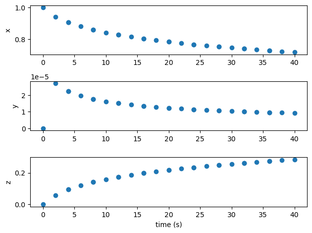
where \(x\), \(y\) and \(z\) are arbitrary states. The initial conditions are

(88)\[\begin{align} x_0 &= 1 \\ y_0 &= z_0 = 0. \end{align}\]

The problem is solved for the time interval \(t\in[0,40)\). There are no controls and constraints.

import numpy as np
import openmdao.api as om

class RobertsonODE(om.ExplicitComponent):
    """example for a stiff ODE from Robertson.
    """

    def initialize(self):
        self.options.declare('num_nodes', types=int)

    def setup(self):
        nn = self.options['num_nodes']

        # input: state
        self.add_input('x', shape=nn, desc="state x", units=None)
        self.add_input('y', shape=nn, desc="state y", units=None)
        self.add_input('z', shape=nn, desc="state z", units=None)
        
        # output: derivative of state
        self.add_output('xdot', shape=nn, desc='derivative of x', units="1/s")
        self.add_output('ydot', shape=nn, desc='derivative of y', units="1/s")
        self.add_output('zdot', shape=nn, desc='derivative of z', units="1/s")

        r = np.arange(0, nn)
        self.declare_partials(of='*', wrt='*', method='exact',  rows=r, cols=r)

    def compute(self, inputs, outputs):

        x = inputs['x']
        y = inputs['y']
        z = inputs['z']

        xdot = -0.04 * x + 1e4 * y * z
        zdot = 3e7 * y ** 2
        ydot = - ( xdot + zdot )
        
        outputs['xdot'] = xdot
        outputs['ydot'] = ydot
        outputs['zdot'] = zdot
        

    def compute_partials(self, inputs, jacobian):

        # x = inputs['x']  # x is not needed to compute partials
        y = inputs['y']
        z = inputs['z']

        xdot_y = 1e4 * z
        xdot_z = 1e4 * y

        zdot_y = 6e7 * y


        jacobian['xdot', 'x'] = -0.04
        jacobian['xdot', 'y'] = xdot_y
        jacobian['xdot', 'z'] = xdot_z

        jacobian['ydot', 'x'] = 0.04
        jacobian['ydot', 'y'] = - ( xdot_y + zdot_y )
        jacobian['ydot', 'z'] = - xdot_z

        jacobian['zdot', 'x'] = 0.0
        jacobian['zdot', 'y'] = zdot_y
        jacobian['zdot', 'z'] = 0.0

Building and running the problem

Here we’re using the ExplicitShooting transcription in Dymos. The ExplicitShooting transcription explicit integrates the given ODE using the solve_ivp method of scipy.

Since this is purely an integration with no controls to be determined, a single call to run_model will propagate the solution for us. There’s no need to run a driver. Even the typical follow-up call to traj.simulate is unnecessary.

Technically, we could even solve this using a single segment since segment spacing in the explicit shooting transcription determines the density of the control nodes, and there are no controls for this simulation. Providing more segments in this case (or a higher segment order) increases the number of nodes at which the outputs are provided.

import openmdao.api as om
import dymos as dm

def robertson_problem(t_final=1.):
    #
    # Initialize the Problem
    #
    p = om.Problem(model=om.Group())
    
    #
    # Create a trajectory and add a phase to it
    #
    traj = p.model.add_subsystem('traj', dm.Trajectory())
    
    tx = dm.ExplicitShooting(num_segments=10, method='LSODA')

    phase = traj.add_phase('phase0',
                           dm.Phase(ode_class=RobertsonODE, transcription=tx))

    #
    # Set the variables
    #
    phase.set_time_options(fix_initial=True, fix_duration=True)

    phase.add_state('x0', fix_initial=True, fix_final=False, rate_source='xdot', targets='x')
    phase.add_state('y0', fix_initial=True, fix_final=False, rate_source='ydot', targets='y')
    phase.add_state('z0', fix_initial=True, fix_final=False, rate_source='zdot', targets='z')

    #
    # Setup the Problem
    #
    p.setup(check=True)

    #
    # Set the initial values
    #

    phase.set_time_val(initial=0.0, duration=t_final)
    phase.set_state_val('x0', [1.0, 0.7])
    phase.set_state_val('y0', [0.0, 1e-5])
    phase.set_state_val('z0', [0.0, 0.3])

    return p

# just set up the problem, test it elsewhere
p = robertson_problem(t_final=40)

p.run_model()

--- Constraint Report [traj] ---
    --- phase0 ---
        None

INFO: checking out_of_order...

INFO:     out_of_order check complete (0.000265 sec).

INFO: checking system...

INFO:     system check complete (0.000019 sec).

INFO: checking solvers...

INFO:     solvers check complete (0.000161 sec).

INFO: checking dup_inputs...

INFO:     dup_inputs check complete (0.000031 sec).

INFO: checking missing_recorders...

WARNING: The Problem has no recorder of any kind attached

INFO:     missing_recorders check complete (0.000565 sec).

INFO: checking unserializable_options...

INFO:     unserializable_options check complete (0.002241 sec).

INFO: checking comp_has_no_outputs...

INFO:     comp_has_no_outputs check complete (0.000022 sec).

INFO: checking auto_ivc_warnings...

INFO:     auto_ivc_warnings check complete (0.000003 sec).

import matplotlib.pyplot as plt

t = p.get_val('traj.phase0.timeseries.time')

states = ['x0', 'y0', 'z0']
fig, axes = plt.subplots(len(states), 1)
for i, state in enumerate(states):
    axes[i].plot(t, p.get_val(f'traj.phase0.timeseries.{state}'), 'o')
    axes[i].set_ylabel(state[0])
axes[-1].set_xlabel('time (s)')
plt.tight_layout()
plt.show()