Analytic Phases in Dymos#
In certain situations analytic solutions are known for the ODE. Typically such situations arise when higher fidelity isn’t needed, but these include:
analytic propagation of a two-body orbit
the Breguet-range equations for an aircraft in steady flight.
In these situations it can be advantageous to utilize the analytic solution and simplify the trajectory optimization problem.
Such phases are avaialble in dymos through the AnalyticPhase class.
Compared to implicit approaches this reduces the size of the optimization problem by removing some design variables and corresponding defect constraints.
Compared to explicit approaches it removes the need to numerically propagate the ODE, which is generally a performance bottleneck.
For analytic phases, the OpenMDAO system we provide to the phase provides the solution to the ODE, not the ODE itself.
where \(\textbf x\) is the vector of state variables (the variable being integrated), \(t\) is time (or time-like), \(\textbf p\) is the vector of parameters (an input to the ODE), and \(\textbf f\) is the ODE solution function.
Differences with other transcriptions#
Note that AnalyticPhase differ from other phases in dymos in a few key ways.
First, the states themselves are purely outputs of the ODE solution function.
This means that the values of the states are never used as design variables, and therefore things like lower and upper bounds or scalers have no meaning.
It is an error to provide these options to a state in an analytic phase.
There is generally no analytic solution to a system when a general time-varying control is provided as an input to the ODE, so they are not permitted to be used with AnalyticPhase. All outputs of the ODE must be based on the values of static parameters and the independent variable (generally time).
AnalyticPhase has the notion of states but they are generally just “special” outputs of the ODE solution system. They are automatically added to the timeseries output with the name {path.to.phase}.states:{state_name}.
Finally, AnalyticPhase doesn’t have the notion of a multi-segment grid on which the solution is calculated.
To keep things as simple as possible, the user provides the phase with a number of nodes at which the solution is requested (lets call it N for now).
Dymos then provides the solution at N Legendre-Gauss-Lobatto (LGL) nodes.
This design decision was made because phase types use the LGL nodes to define the input times of polynomial control variables.
This means that values of an output of an AnalyticPhase can be fed into another phase as a polynomial control.
- AnalyticPhase.add_state(name, state_name=None, units=unspecified, shape=unspecified)[source]
Add a state variable to be integrated by the phase.
- Parameters:
- namestr
Path to use as the source of the state variable.
- state_namestr
Name of the state variable, if the last element of the source path is ambiguous.
- unitsstr or None
Units in which the state variable is defined. If units is not specified here then the unit will be determined from the source.
- shapetuple of int
The shape of the state variable. For instance, a 3D cartesian position vector would have a shape of (3,).
A basic example#
Suppose we want to use Dymos to solve the ODE
subject to:
Here we want to find the value of x at t=2.
We can absolutely use a pseudospectral method or explicit shooting in Dymos to find the value of x on a given interval using this information. But in this case, the solution is known analytically.
We need to find the value of constant \(c_1\) to find our particular solution. Applying the given initial condition gives c_1 as 0.
The component that provides the solution is then:
import numpy as np
import matplotlib.pyplot as plt
import openmdao.api as om
import dymos as dm


class SimpleIVPSolution(om.ExplicitComponent):

    def initialize(self):
        self.options.declare('num_nodes', types=(int,))

    def setup(self):
        nn = self.options['num_nodes']
        self.add_input('t', shape=(nn,), units='s')
        self.add_input('x0', shape=(1,), units='unitless', tags=['dymos.static_target'])
        self.add_output('x', shape=(nn,), units='unitless')

        ar = np.arange(nn, dtype=int)
        self.declare_partials(of='x', wrt='t', rows=ar, cols=ar)
        self.declare_partials(of='x', wrt='x0')

    def compute(self, inputs, outputs):
        t = inputs['t']
        x0 = inputs['x0']
        outputs['x'] = t ** 2 + 2 * t + 1 - x0 * np.exp(t)

    def compute_partials(self, inputs, partials):
        t = inputs['t']
        x0 = inputs['x0']
        partials['x', 't'] = 2 * t + 2 - x0 * np.exp(t)
        partials['x', 'x0'] = -np.exp(t)
Solving the problem with Dymos looks like this
p = om.Problem()
traj = p.model.add_subsystem('traj', dm.Trajectory())
phase = dm.AnalyticPhase(ode_class=SimpleIVPSolution, num_nodes=10)
traj.add_phase('phase', phase)
phase.set_time_options(units='s', targets=['t'], fix_initial=True, fix_duration=True)
phase.add_state('x')
phase.add_parameter('x0', opt=False)
p.setup()
phase.set_time_val(0.0, 2.0, units='s')
phase.set_parameter_val('x0', 0.5, units='unitless')
p.run_model()
t = p.get_val('traj.phase.timeseries.time', units='s')
x = p.get_val('traj.phase.timeseries.x', units='unitless')
print(f'x({t[-1, 0]}) = {x[-1, 0]}')
# A dense version of the analytic solution for plot comparison.
def expected(time):
return time ** 2 + 2 * time + 1 - 0.5 * np.exp(time)
t_dense = np.linspace(t[0], t[-1], 100)
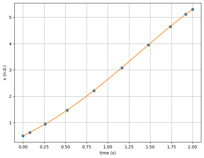
plt.subplots(1, 1, figsize=(8, 6))
plt.plot(t, x, 'o')
plt.plot(t_dense, expected(t_dense), '-')
plt.xlabel('time (s)')
plt.ylabel('x (n.d.)')
plt.grid()
plt.show()
x(2.0) = 5.305471950534675
Possible Questions#
You might be asking
Why use Dymos at all here? This is just as easy to do with a pure OpenMDAO component.
And you’d be absolutely right. But what makes this useful in the context of Dymos is that it allows us to pose a trajectory as the continuous evolution of a system in time. Often in real practice we have portions of a trajectory where an analytic solution is available, and by utilizing an analytic solution to obtain the output in those phases, we make the problem easier for the optimizer to solve.
Why not allow the initial state value to be an input to the phase?
We had considered having the initial state value be a variable in this case, but it was a construct that didn’t mesh well with the other transcriptions.
It would require the addition of an initial_state_targets option that wouldn’t apply to other transcriptions.
Also, the particular solution is often, but not always found using the value of the state at the initial time.
In these cases, using a generic parameter felt like the more flexible way of doing things while minimizing changes to the existing code.
Additional differences#
Since AnalyticPhases only output state values, there is no notion of a target of state variable in an AnalyticPhase.
In an AnalyticPhase, states need a source.
Much like timeseries outputs, when we add a state to the AnalyticPhase we can specify the entire path, and the last bit of the path (after the last period) will be used for the name of the state.
And just as add_timeseries_output uses argument output_name to disambiguate the name of the timeseries output if necessary, add_state will accept state_name if the last portion of the path is ambiguous.
Linking Analytic Phases#
AnalyticPhase provides timeseries output and so it can be linked to other phases using continuity constraints. However, since the initial value of the state is not an input variable in the phase it does not support linking with option connected = True.
In the example below, we add an intermediate breakpoint to the solution above where \(x = 1.5\).
Changing the connected argument of link_phases to True will raise an error.
p = om.Problem()
traj = p.model.add_subsystem('traj', dm.Trajectory())

first_phase = dm.AnalyticPhase(ode_class=SimpleIVPSolution, num_nodes=10)
first_phase.set_time_options(units='s', targets=['t'], fix_initial=True, duration_bounds=(0.5, 10.0))
first_phase.add_state('x')
first_phase.add_parameter('x0', opt=False)

first_phase.add_boundary_constraint('x', loc='final', equals=1.5, units='unitless')

second_phase = dm.AnalyticPhase(ode_class=SimpleIVPSolution, num_nodes=10)
second_phase.set_time_options(units='s', targets=['t'], duration_bounds=(0.1, 10.0))
second_phase.add_state('x')
second_phase.add_parameter('x0', opt=False)

second_phase.add_boundary_constraint('time', loc='final', equals=2.0, units='s')

# Since we're using constraints to enforce continuity between the two phases, we need a
# driver and a dummy objective.  As usual, time works well for a dummy objective here.
first_phase.add_objective('time', loc='final')
p.driver = om.ScipyOptimizeDriver()

traj.add_phase('first_phase', first_phase)
traj.add_phase('second_phase', second_phase)

# We can link time with a connection, since initial time is an input to the second phase.
traj.link_phases(['first_phase', 'second_phase'], ['time'], connected=True)
Different ways to handle the phase linkage for state continuity#
At this point we need to choose how to enforce state continuity.
We cannot simply use traj.link_phases(['first_phase', 'second_phase'], ['x'], connected=True) because the initial value of state x is not an input to the phase.
One might think to link state x from first_phase to parameter x0 from second phase, but that is also not correct, because x0 is not the initial value of x in the phase but the value of x at t=0.
We could redefine x0 to be the value at the initial time, however.
Valid options here would be to link the states together with unconnected phases, using a constraint:
traj.link_phases(['first_phase', 'second_phase'], ['x'], connected=False)
Alternatively, we could either link parameters x0 together in both phases (a connection would be fine) or use a trajectory-level parameter to pass a single value of x0 to both phases.
In the example below, trajectory parameter x0 is fed to the parameter of the same name in the phases.
You’ll need to make sure that both of the target parameters are not designated as design variables (opt = False).
traj.add_parameter('x0', val=0.5, opt=False)
p.setup()
first_phase.set_time_val(0.0, 2.0, units='s')
p.set_val('traj.parameters:x0', 0.5, units='unitless')
p.run_driver()
t_1 = p.get_val('traj.first_phase.timeseries.time', units='s')[:, 0]
x_1 = p.get_val('traj.first_phase.timeseries.x', units='unitless')[:, 0]
x0_1 = p.get_val('traj.first_phase.parameter_vals:x0')[:, 0]
t_2 = p.get_val('traj.second_phase.timeseries.time', units='s')[:, 0]
x_2 = p.get_val('traj.second_phase.timeseries.x', units='unitless')[:, 0]
x0_2 = p.get_val('traj.second_phase.parameter_vals:x0')[:, 0]
print(f'x({t_1[-1]}) = {x_1[-1]}')
print(f'x({t_2[-1]}) = {x_2[-1]}')
# A dense version of the analytic solution for plot comparison.
def expected(time):
return time ** 2 + 2 * time + 1 - x0_1 * np.exp(time)
t_dense = np.linspace(t_1[0], t_2[-1], 100)
plt.subplots(1, 1, figsize=(8, 6))
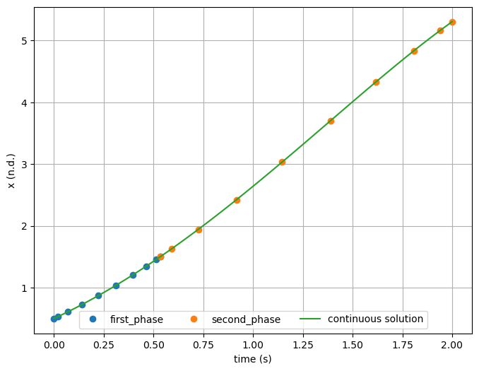
plt.plot(t_1, x_1, 'o', label='first_phase')
plt.plot(t_2, x_2, 'o', label='second_phase')
plt.plot(t_dense, expected(t_dense), '-', label='continuous solution')
plt.xlabel('time (s)')
plt.ylabel('x (n.d.)')
plt.grid()
plt.legend(ncol=3, loc='lower center')
plt.show()
Optimization terminated successfully    (Exit mode 0)
            Current function value: 0.533871279941519
            Iterations: 4
            Function evaluations: 4
            Gradient evaluations: 4
Optimization Complete
-----------------------------------
x(0.533871279941519) = 1.5000000542207101
x(2.0) = 5.305471950534675