Boundary Balance

In some cases, using dymos without the need for an optimizer is desirable. Sometimes in the absense of a control, you may just want to propagate the problem. Solve segments allows us to do this for a specified amount of time, but if the duration of the phase is itself an implicit output, then we need dymos to understand the residual to associate with the phase duration.

This feature requires that some output of the system is directly coupled to one of the phase parameters, such as t_duration. In a collocation phase where an optimizer satisfies the defect equations, changing the duration of the phase does not directly impact the final conditions of the system. The transcription needs to be such that invoking run_model is enough to generate outputs that change with the desired parameters. The transcription must be one of ExplicitShooting, PicardShooting, or a pseudospectral transcription with solve_segments=True.

Solving the brachistochrone without an optimizer.

import numpy as np
import openmdao.api as om


class BrachistochroneODE(om.ExplicitComponent):
    """
    The brachistochrone EOM assuming
    """

    def initialize(self):
        self.options.declare('num_nodes', types=int)

    def setup(self):
        nn = self.options['num_nodes']

        # static parameters
        self.add_input('v', desc='speed of the bead on the wire', shape=(nn,), units='m/s')
        self.add_input('theta', desc='angle between wire tangent and the nadir', shape=(nn,), units='rad')
        self.add_input('g', desc='gravitational acceleration', shape=(1,), tags=['dymos.static_target'], units='m/s**2')

        self.add_output('xdot', desc='velocity component in x', shape=(nn,), units='m/s',
                        tags=['dymos.state_rate_source:x', 'dymos.state_units:m'])

        self.add_output('ydot', desc='velocity component in y', shape=(nn,), units='m/s',
                        tags=['dymos.state_rate_source:y', 'dymos.state_units:m'])

        self.add_output('vdot', desc='acceleration magnitude', shape=(nn,), units='m/s**2',
                        tags=['dymos.state_rate_source:v', 'dymos.state_units:m/s'])

        self.declare_coloring(method='cs')

    def compute(self, inputs, outputs):
        v, theta, g = inputs.values()

        sin_theta = np.sin(theta)
        cos_theta = np.cos(theta)

        outputs['vdot'] = g * cos_theta
        outputs['xdot'] = v * sin_theta
        outputs['ydot'] = -v * cos_theta

Propagating the equations of motion using solve_segments

In the following example, we set solve_segments='forward' such that all of the collocation defects associate with the Radau transcription are satisfied by a Newton solver rather than the optimizer. This is the first step to solving the problem without an optimizer. This ensures that the equations of motion are satisfied to the extent possible assuming the transcription grid.

In pseudospectral phases, solve_segments is an optional setting that can be applied to all states in the phase via the solve_segments option on the pseudospectral transcriptions, or to individual states.

In phases that use PicardShooting, solve_segments must be 'forward' or 'backward'. The default direction of the solve is 'forward', but individual states may override this.

You can experiment with using different transcriptions below by choosing which value of TX you want to use. Note that because the initial states of the brachistochrone are fixed, solve_segments='forward' should be used.

# TX = dm.PicardShooting(num_segments=5, nodes_per_seg=4, solve_segments='forward')
TX = dm.Radau(num_segments=10, order=3, solve_segments='forward', compressed=True)
# TX = dm.ExplicitShooting(num_segments=10, order=3)

# Define the OpenMDAO problem
p = om.Problem(model=om.Group())

# Define a Trajectory object
traj = dm.Trajectory()
p.model.add_subsystem('traj', subsys=traj)

# Define a Dymos Phase
phase = dm.Phase(ode_class=BrachistochroneODE,
                 transcription=TX)
traj.add_phase(name='phase0', phase=phase)

# Set the time options
phase.set_time_options(fix_initial=True,
                       duration_bounds=(0.5, 10.0))

# Set the state options
phase.add_state('x', rate_source='xdot',
                fix_initial=True)
phase.add_state('y', rate_source='ydot',
                fix_initial=True)
phase.add_state('v', rate_source='vdot',
                fix_initial=True)

phase.add_control('theta', lower=0.0, upper=1.5, units='rad')
phase.add_parameter('g', opt=False, val=9.80665, units='m/s**2')

# Minimize final time.
phase.add_objective('time', loc='final')

# Set the driver.
p.driver = om.ScipyOptimizeDriver()

# Allow OpenMDAO to automatically determine our sparsity pattern.
# Doing so can significant speed up the execution of dymos.
p.driver.declare_coloring()

phase.nonlinear_solver = om.NewtonSolver(maxiter=100, solve_subsystems=True, stall_limit=3, iprint=2)
phase.linear_solver = om.DirectSolver()

# Setup the problem
p.setup()

phase.set_time_val(initial=0.0, duration=2.0)
phase.set_state_val('x', vals=[0, 10])
phase.set_state_val('y', vals=[10, 5])
phase.set_state_val('v', vals=[0.1, 100])
phase.set_control_val('theta', vals=[0.0, 90.0], units='deg')
phase.set_parameter_val('g', val=9.80665)

# Run the driver to solve the problem
p.run_model()

==================
traj.phases.phase0
==================
NL: Newton 0 ; 37.4386489 1

Coloring for 'traj.phases.phase0.rhs_all' (class BrachistochroneODE)

Jacobian shape: (120, 81)  (2.47% nonzero)
FWD solves: 2   REV solves: 0
Total colors vs. total size: 2 vs 81  (97.53% improvement)

Sparsity computed using tolerance: 1e-25.
Dense partial jacobian for BrachistochroneODE 'traj.phases.phase0.rhs_all' was computed 3 times.
Time to compute sparsity:   0.0077 sec
Time to compute coloring:   0.0078 sec
Memory to compute coloring:   0.2500 MB
NL: Newton 1 ; 3.98269488e-12 1.06379236e-13
NL: Newton Converged

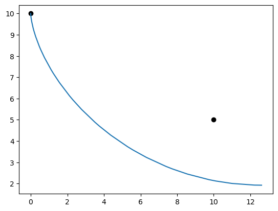
If we plot the resulting trajectory of the bead, we notice that our guesses for time and the control history didn’t bring the bead to the desired target at (10, 5):

%matplotlib inline
import matplotlib.pyplot as plt

x = p.get_val('traj.phase0.timeseries.x')
y = p.get_val('traj.phase0.timeseries.y')

plt.plot(0.0, 10.0, 'ko')
plt.plot(10.0, 5.0, 'ko')
plt.plot(x, y)
plt.show()

Stopping the propagation at the desired time.

We can utilize the add_boundary_balance method on Phase to turn t_duration into an implicit output and provide it with a residual.

In our case, we set phase.add_boundary_balance(param='t_duration', name='x', tgt_val=10.0)

This specifies that we want t_duration to be associated with the following residual:

(96)\[\begin{align} \mathcal{R}(t_d) = x - 10 = 0 \end{align}\]

Note that we limit the angle \(\theta\) to be between 0 and 180, the bead must move to the right and we can just terminate the propagation when x=10.

#TX = dm.PicardShooting(num_segments=5, nodes_per_seg=4, solve_segments='forward')
TX = dm.Radau(num_segments=10, order=3, solve_segments='forward', compressed=True)
# TX = dm.ExplicitShooting(num_segments=10, order=3)

# Define the OpenMDAO problem
p = om.Problem(model=om.Group())

# Define a Trajectory object
traj = dm.Trajectory()
p.model.add_subsystem('traj', subsys=traj)

# Define a Dymos Phase
phase = dm.Phase(ode_class=BrachistochroneODE,
                 transcription=TX)
traj.add_phase(name='phase0', phase=phase)

# Set the time options
phase.set_time_options(fix_initial=True)
phase.add_boundary_balance(param='t_duration', name='x', tgt_val=10.0)

# Set the state options
phase.add_state('x', rate_source='xdot',
                fix_initial=True)
phase.add_state('y', rate_source='ydot',
                fix_initial=True)
phase.add_state('v', rate_source='vdot',
                fix_initial=True)

phase.add_control('theta', lower=0.0, upper=1.5, units='rad')
phase.add_parameter('g', opt=False, val=9.80665, units='m/s**2')

# Minimize final time.
phase.add_objective('time', loc='final')

# Set the driver.
p.driver = om.ScipyOptimizeDriver()

# Allow OpenMDAO to automatically determine our sparsity pattern.
# Doing so can significant speed up the execution of dymos.
p.driver.declare_coloring()

phase.nonlinear_solver = om.NewtonSolver(maxiter=1000, solve_subsystems=True, stall_limit=3)
phase.nonlinear_solver.linesearch = None
phase.linear_solver = om.DirectSolver()

# Setup the problem
p.setup()

phase.set_time_val(initial=0.0, duration=1.8)
phase.set_state_val('x', vals=[0, 10])
phase.set_state_val('y', vals=[10, 5])
phase.set_state_val('v', vals=[0.1, 100])
phase.set_control_val('theta', vals=[0.0, 90.0], units='deg')
phase.set_parameter_val('g', val=9.80665)

# Run the driver to solve the problem
p.run_model()

==================
traj.phases.phase0
==================

Coloring for 'traj.phases.phase0.rhs_all' (class BrachistochroneODE)

Jacobian shape: (120, 81)  (2.47% nonzero)
FWD solves: 2   REV solves: 0
Total colors vs. total size: 2 vs 81  (97.53% improvement)

Sparsity computed using tolerance: 1e-25.
Dense partial jacobian for BrachistochroneODE 'traj.phases.phase0.rhs_all' was computed 3 times.
Time to compute sparsity:   0.0071 sec
Time to compute coloring:   0.0077 sec
Memory to compute coloring:   0.0000 MB
NL: Newton Converged in 4 iterations

%matplotlib inline
import matplotlib.pyplot as plt

x = p.get_val('traj.phase0.timeseries.x')
y = p.get_val('traj.phase0.timeseries.y')
v = p.get_val('traj.phase0.timeseries.y')
theta = p.get_val('traj.phase0.timeseries.theta')

plt.plot(0.0, 10.0, 'ko')
plt.plot(10.0, 5.0, 'ko')
plt.plot(x, y)
plt.show()

print('final time', p.get_val('traj.phase0.timeseries.time')[-1])
print('final y', y[-1])
print('final theta', np.degrees(theta[-1]))

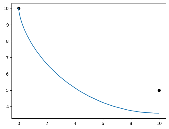
final time [1.7796735]
final y [3.59263225]
final theta [90.]

Solving the brachistochrone without an optimizer

The brachistochrone has an analytic solution such that rate of change of the tangent to the wire (angle $\theta) is constant. We can use this information to pose the brachistochrone as a boundary value problem and solve as a shooting problem.

We add another implicit output that provides the rate of change as a constant value throughout the trajectory. That means that theta_rate is a parameter as far as dymos is concerned. We then make theta a state variable whose rate is provided by the theta_rate parameter. We’ll set the initial value of theta to zero degrees, since we know that is approximately correct for this problem.

(97)\[\begin{align} \mathcal{R}(\dot{\theta}) &= y_f - 5 \end{align}\]

Dymos currently doesn’t support making parameters implicit outputs, so we’re going to do this the manual OpenMDAO way.

# TX = dm.PicardShooting(num_segments=5, nodes_per_seg=4, solve_segments='forward')
TX = dm.Radau(num_segments=10, order=3, solve_segments='forward', compressed=True)
# TX = dm.ExplicitShooting(num_segments=10, order=3)

# Define the OpenMDAO problem
p = om.Problem(model=om.Group())

# Define a Trajectory object
traj = dm.Trajectory()
p.model.add_subsystem('traj', subsys=traj)

# Define a Dymos Phase
phase = dm.Phase(ode_class=BrachistochroneODE,
                 transcription=TX)
traj.add_phase(name='phase0', phase=phase)

# Set the time options
phase.set_time_options(fix_initial=True)

# Set the state options
phase.add_state('x', rate_source='xdot',
                fix_initial=True)
phase.add_state('y', rate_source='ydot',
                fix_initial=True)
phase.add_state('v', rate_source='vdot',
                fix_initial=True)
phase.add_state('theta', rate_source='theta_rate',
                fix_initial=True, units='rad')

phase.add_parameter('theta_rate', opt=False, units='rad/s')
phase.add_parameter('g', opt=False, val=9.80665, units='m/s**2')

# Minimize final time.
phase.add_objective('time', loc='final')

# Set the driver.
p.driver = om.ScipyOptimizeDriver()

# Allow OpenMDAO to automatically determine our sparsity pattern.
# Doing so can significant speed up the execution of dymos.
p.driver.declare_coloring()

phase.nonlinear_solver = om.NewtonSolver(maxiter=1000, solve_subsystems=True, stall_limit=3,
                                         iprint=0, atol=1.0E-8, rtol=1.0E-8, debug_print=True)
phase.nonlinear_solver.linesearch = None
phase.linear_solver = om.DirectSolver()

# Define balance residuals to be converged by varying t_duration and theta_rate.
phase.add_boundary_balance('t_duration', name='x', tgt_val=10.0, loc='final', eq_units='m')
phase.add_boundary_balance('theta_rate', name='y', tgt_val=5.0, loc='final', eq_units='m')

# Now we need a solver to converge the loop around the entire problem.
p.model.nonlinear_solver = om.NewtonSolver(maxiter=100, solve_subsystems=True, stall_limit=3,
                                           iprint=0, atol=1.0E-8, rtol=1.0E-8, debug_print=True)
p.model.nonlinear_solver.linesearch = None
p.model.linear_solver = om.DirectSolver()

# Setup the problem
p.setup()

phase.set_time_val(initial=0.0, duration=1.8)
phase.set_state_val('x', vals=[0, 10])
phase.set_state_val('y', vals=[10, 5])
phase.set_state_val('v', vals=[0., 10])
phase.set_state_val('theta', vals=[0.0, 45], units='deg')
phase.set_parameter_val('g', val=9.80665)

# Note that we set theta_rate at the balance comp, which is then passed into the phase as a parameter.
phase.set_parameter_val('theta_rate', 0.5, units='rad/s')

# Run the driver to solve the problem
p.run_model()

Coloring for 'traj.phases.phase0.rhs_all' (class BrachistochroneODE)

Jacobian shape: (120, 81)  (2.47% nonzero)
FWD solves: 2   REV solves: 0
Total colors vs. total size: 2 vs 81  (97.53% improvement)

Sparsity computed using tolerance: 1e-25.
Dense partial jacobian for BrachistochroneODE 'traj.phases.phase0.rhs_all' was computed 3 times.
Time to compute sparsity:   0.0071 sec
Time to compute coloring:   0.0076 sec
Memory to compute coloring:   0.0000 MB

%matplotlib inline
import matplotlib.pyplot as plt

x = p.get_val('traj.phase0.timeseries.x')
y = p.get_val('traj.phase0.timeseries.y')
v = p.get_val('traj.phase0.timeseries.y')
theta = p.get_val('traj.phase0.timeseries.theta')

plt.plot(0.0, 10.0, 'ko')
plt.plot(10.0, 5.0, 'ko')
plt.plot(x, y)
plt.show()

print('final time', p.get_val('traj.phase0.timeseries.time')[-1])
print('final y', y[-1])
print('final theta', np.degrees(theta[-1]))

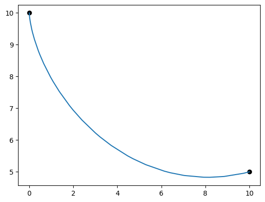
final time [1.80160313]
final y [5.]
final theta [100.50736083]

Using a combination of solve_segments and boundary balances, we’ve managed to solve the brachistochrone problem without the need of an optimizer.

Note that solving problems in this way can be filled with pitfalls. Here we have a formulation of the brachistochrone that is robust to a variety of values for the parameter theta_rate. An alternative formulation is to keep the ratio \(\frac{\sin{\theta}}{v}\) constant. However, using the inverse sine in that formulation can easily result in domain issues which makes convergence difficult.

Unlike solve_segments options in pseudospectral phases, the PicardShooting method uses multiple levels of solvers. The inner-most solver converges the state history in each segment. Outside of that a “multiple shooting” solver ensures state continuity between segments within a phase. Finally, the entire phase uses a NewtonSolver to find the value of any “boundary balance” outputs by driving their associated residuals to zero. In some situations